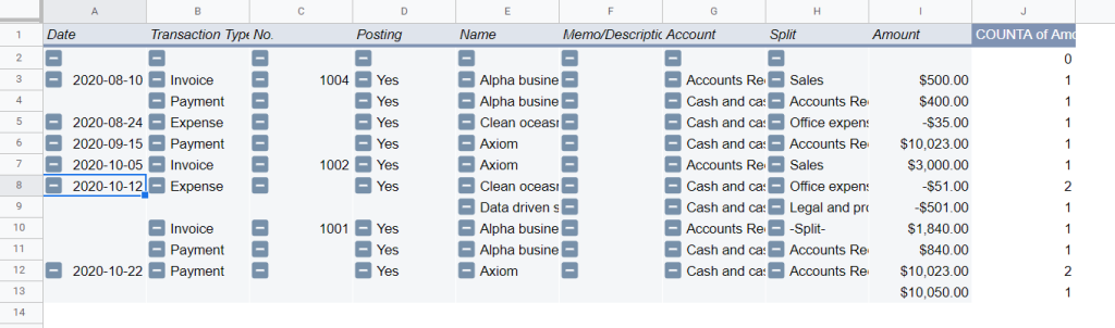
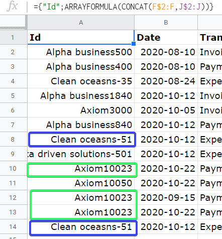
Imagine the following: you have imported data from your database to Google Sheets to create a report. While scanning through the entries, you spotted that some of them are duplicated like this:
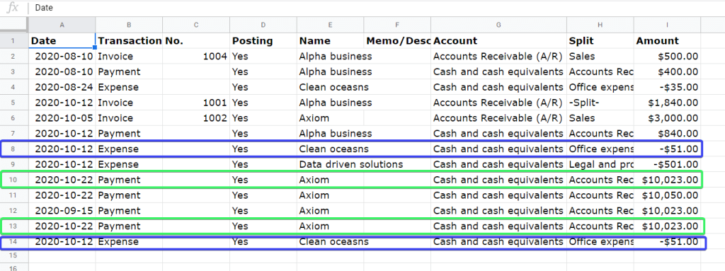
Would you remove the duplicate rows manually? This could be an option, but if your data set is large enough, you’d better automate the removal. In this guide, we’ll show you all the possible options to delete duplicates in Google Sheets docs using native functionality, formulas, or tricky workarounds.
Remove duplicate rows in Google Sheets in five steps
To remove duplicate values in Google Sheets you don’t need to manually delete each duplicate row. Google Sheets can do this for you with literally five steps:
- Select the range of cells that you want to clear from duplicates.
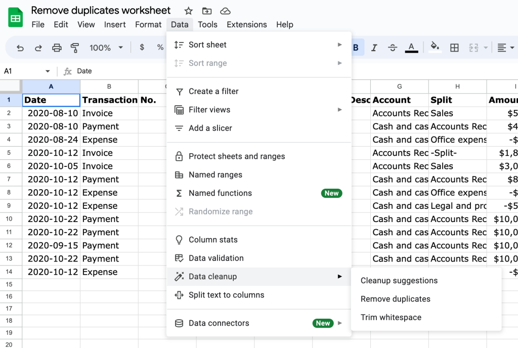
- Go to the Data menu => Data cleanup => Remove duplicates.
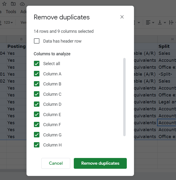
- Check whether the selected data range has a header row.
- Select the columns to analyze for duplicates.
- Click Remove duplicates.
It works like a charm, see yourself in the following example.
Example of duplicates removal in Google Sheets
For example, you want to remove entries that have a duplicate name or date. Select the range of cells and use the following path: Data menu => Data cleanup => Remove duplicates.
In our case, we selected all these columns since we want to totally remove duplicate values in Google Sheets.
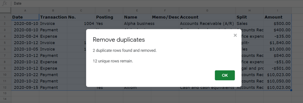
The next moment, the duplicate rows have been removed successfully.
This functionality will work for larger data sets as well. However, its main drawback is that you’ll have to manually repeat it each time you add new entries to the data set. And what if you have added more than 50 entries and you’re not sure whether there are any duplicates in your Google Sheets doc? Below, you’ll find the solutions to automate the identification and removal of duplicate entries.
Remove duplicates Google Sheets: what are the options
Apart from the built-in tool to get rid of duplicate data in Google Sheets, you can make use of the following options:
- Google Sheets functions – use formulas to remove duplicate rows.
- Pivot tables – change the view of your data set and hide the duplicate cells.
- Apps Script – create custom functions that will remove duplicate values based on the preset conditions.
- Google Sheets add-ons – on the Google Workspace Marketplace, you can find a few solutions to remove duplicates.
And what about conditional formatting? Some say that you can use it to remove duplicate entries in Google Sheets as well. Actually, conditional formatting only allows you to highlight duplicates. The removal part still has to be done manually with the native remove duplicates tool.
Check out the potential cases to remove duplicates in Google Sheets and the best options to solve them.
How to remove duplicates in one column in Google Sheets
When you are dealing with a single column or an integral data range, the UNIQUE function is the best option to remove duplicates. You’ll need one formula to do the job.
Alternatively, you can identify duplicates using the COUNTIF function in a separate column, or even highlight them using Conditional Formatting Google Sheets. Then you’ll be able to remove them manually or by using the Remove Duplicates functionality. Jump to the needed section if this is what you need.
How to remove duplicates in Google Sheets from 2 or more different columns
This requires a more advanced approach, and you can benefit from multiple solutions:
- Pivot table – it will automatically remove duplicates in a separate sheet
- UNIQUE function – it can remove duplicates from an integral data range
- QUERY function – it’s a bit intricate, but a reliable solution
- Two-step approach – where you first identify duplicates by a unique ID and then remove them using an advanced formula
We would recommend you check out the pivot table first and then move to formula-based options.
How to remove duplicates in Google Sheets but keep their position
The best way to remove duplicates without ruining the order of your data set is to use Conditional Formatting. This option includes two steps:
- Identifying and highlighting duplicates
- Removing duplicates manually
This will take time, but you’ll be able to handle the task as you need to.
If you have a clear vision of which solution will do the job for you, go to the relevant section right away. If you don’t, check out all of them and choose the best one for your needs.
How to remove duplicate cells in Google Sheets using pivot tables
The idea of a pivot table is that you can rotate your data set to view it from a different perspective or reorganize data without changing it. We won’t change the perspective, but simply display data in the pivot table, which identifies and removes duplicates itself as follows:
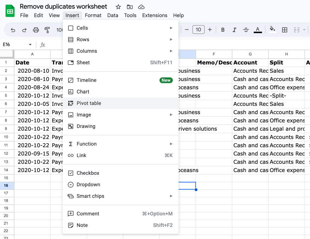
To do this, go to the Insert menu and select Pivot table.
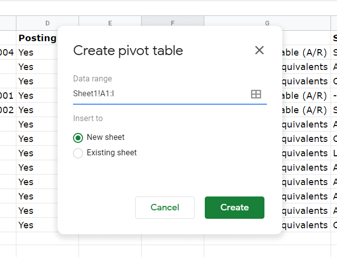
Then select the data range to analyze and specify where the pivot table will be created: either in a new or existing sheet.
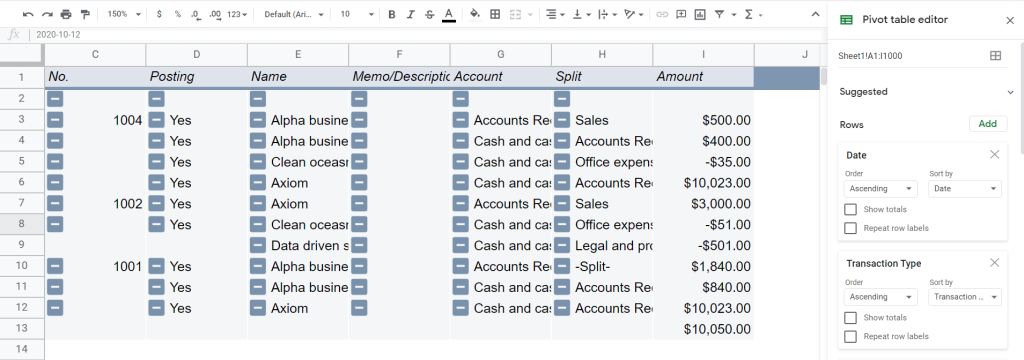
The pivot table was created and you need to set it up using the Pivot table editor that you’ll see on the right of your spreadsheet.
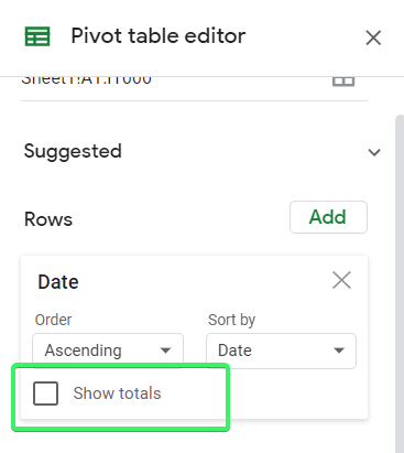
Add rows to your pivot table
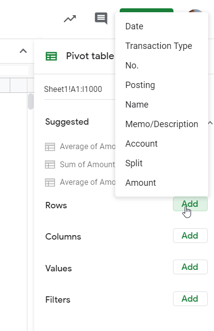
In our example, we wanted to transfer all the columns from our data set. To do this, click Add (Rows section) and select the column. We also unchecked the Show totals checkbox.
You’ll have to repeat this action for each column separately. In the end, you’ll get the pivot table with the duplicates removed:
Add values to your pivot table
If you want to know which entries were duplicated, go to the Values section in the Pivot table editor and click Add.
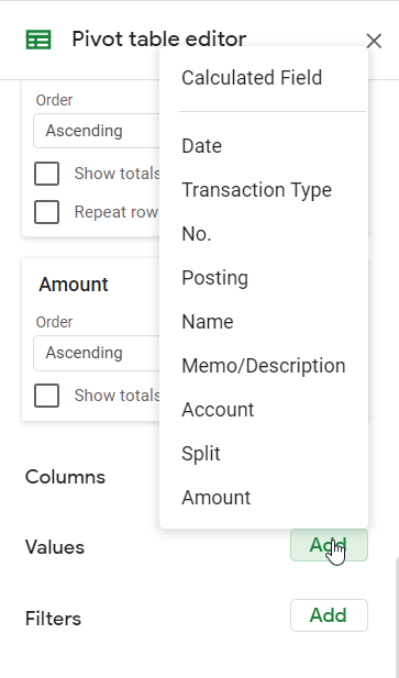
Choose the column (s) to analyze for duplicates and select COUNTA in the Summarize by field. You’ll get a separate column with numbers:
- 1 means that there is one entry
- 2 or more means that this entry was duplicated
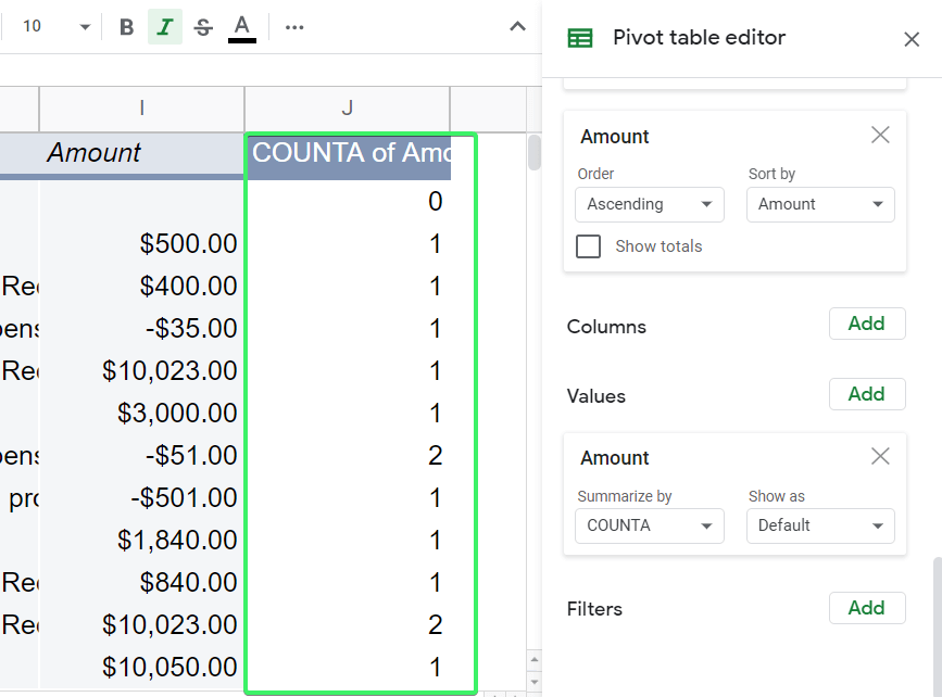
Now if you add new entries to your initial data set, they will be automatically identified in this column and removed in your pivot table.
We have introduced the basic pivot table configuration for this use case. Read our Pivot Table Google Sheets guide to customize it for your needs.
How to delete duplicates in Google Sheets using formulas
Basically, UNIQUE and QUERY are the two functions that you can use to delete duplicate data in Google Sheets. However, there are other options as well. We’ll check them out below.
UNIQUE function in Google Sheets to remove duplicate rows based on one column
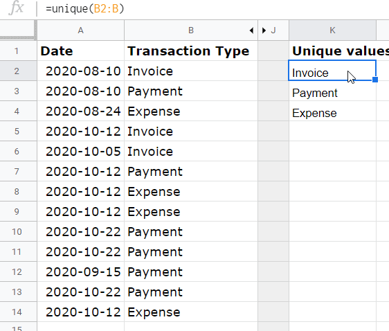
UNIQUE is a Google Sheets function to return unique values from a range by removing duplicates. It has a very simple syntax:
=UNIQUE(data-range)For example, let’s extract unique values from our Transaction Type column (B2:B). Apply the following formula and here we go:
=unique(B2:B)
If you need to remove duplicates based on the analysis of multiple columns, like in our case, UNIQUE will do the job as well. Specify the range to check and it only returns unique rows:
=unique(Sheet1!A1:J)
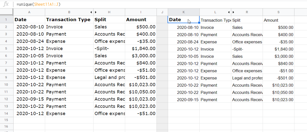
The drawback of the UNIQUE option is that you cannot choose which columns you want to analyze for duplicates. But you can do this with QUERY.
Get rid of duplicates in Google Sheets using the QUERY function
The Google Sheets QUERY function lets you select specific columns of your data set and delete duplicate entries from them. The QUERY formula syntax is the following:
=QUERY(data-range,query)The query to remove duplicates should contain:
- SELECT clause to select the columns you want to query.
- GROUP BY clause to group values across the selected data range. GROUP BY only works if you apply one of the aggregation functions (
avg,count,max,min,sum) within the SELECT clause. - OFFSET or WHERE clause to skip an empty row at the top
Here is how the query may look:
"Select A,min(B),H,I group by A,H,I offset 1"
Let’s check it out with an example. We need to remove duplicates from the same data set that we used above. Another condition is to return only four columns from it: Date, Transaction Type, Split, and Amount. Here is the QUERY formula to do this:
=query(A2:I,"Select A,min(B),H,I group by A,H,I offset 1")
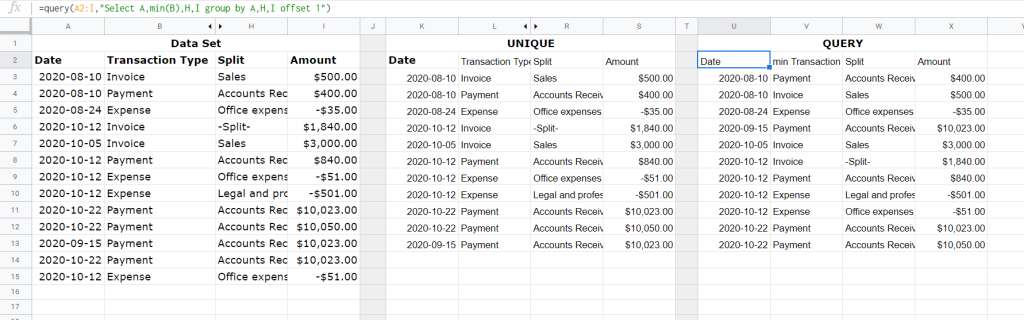
We showed it next to the unique values obtained with the UNIQUE formula, so you can compare the difference. QUERY removed duplicates and returned unique rows but it sorted the entries in descending order. Let’s explain how it worked:
Select A,min(B),H,I– we specified the columns we need.min(B)– we have to apply an aggregation function within the SELECT clause, so we choosemin.group by A,H,I– we specified the columns to group by (the column with the aggregated function cannot be included here).offset 1– we used OFFSET to remove the empty row at the top. Alternatively, you can use the WHERE clause (where A Is not NULL) to exclude entities that have no numeric value.
If the QUERY option is what you need but you think it’s a bit tricky, here’s an alternative solution.
Identify and remove duplicates from Google Sheets on multiple columns using the merging functions
This option consists of two steps:
- Identify duplicates in the columns you want to analyze.
- Remove duplicate entries.
Identify duplicates in your Google Sheets data set
To identify the duplicate entries in specific columns, you’ll need to create a unique identifier based on the values from these columns. Let me explain this with an example.
In our data set, we want to remove duplicates by analyzing two columns: Name and Amount. Note that we exclude the Date column from the analysis.
To make a unique identifier for each entry, you’ll need to merge values from these columns into a single string (one string for each row). To do this, create a new column on the left and apply the following formula:
={"Id";ARRAYFORMULA(CONCAT(F$2:F,J$2:J))}

F$2:F– Name columnJ$2:J– Amount columnCONCAT(F$2:F,J$2:J)– CONCAT formula to merge two values togetherARRAYFORMULA– function to expand the CONCAT formula{"Id";– to assign the column name
As a result, we now have unique IDs that let us identify duplicates easily:
Note: If you need to search for duplicates on more than two columns, the CONCAT function won’t do the job. You can replace it with another function or method to merge data such as &(ampersand), CONCATENATE, JOIN, etc. Read our blog post to learn more about how to merge cells in Google Sheets.
Remove duplicates in Google Sheets using their unique IDs
Create a new sheet where you want only to import the unique rows without duplicates and apply the following formula:
={
  Sheet1!A1:J1;
  SORTN(
       FILTER(Sheet1!A2:J, LEN(Sheet1!A2:A) > 0),
       ROWS(FILTER(Sheet1!A2:J, LEN(Sheet1!A2:A) > 0)),
       2,1,true
  )
}
Sheet1!A2:J– data set with duplicate entriesFILTER(Sheet1!A2:J, LEN(Sheet1!A2:A) > 0)– to exclude empty rows from the initial data setROWS(FILTER(Sheet1!A2:J, LEN(Sheet1!A2:A) > 0))– the number of rows in the initial data setSORTN(...,2,1,true)– to show at most the first n rows after removing duplicate rows and sort by the first column in ascending order{Sheet1!A1:J1– to import column names from the data set with duplicate entries
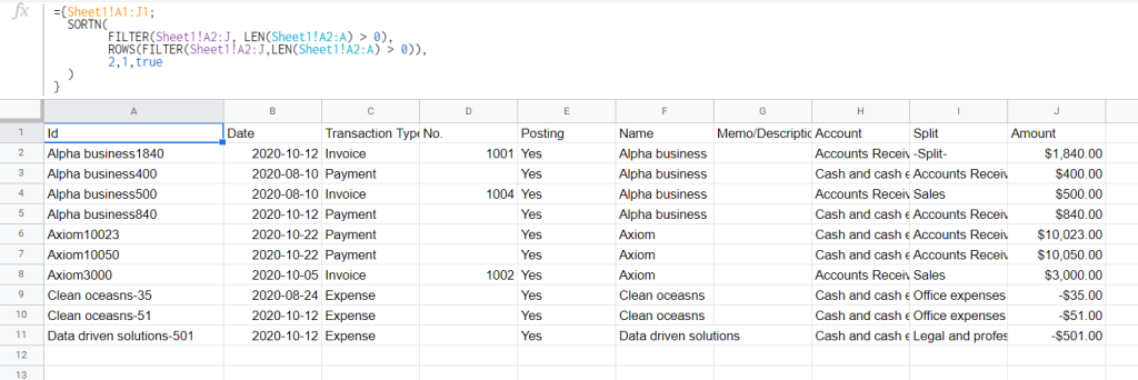
The formula returns the initial data set without duplicates by taking the first occurrence of each row. This method is quite useful if you need to automate deduplication in Google Sheets like in the case below.
Remove duplicate values from the automatically refreshed dataset in Google Sheets
Let’s say you have a spreadsheet that updates automatically with new entries exported from an external source. In our case, we connected Google Sheets to HubSpot with the help of the ETL tool designed by Coupler.io.
Coupler.io is a data automation and analytics platform that empowers organizations to gain the most from their data. It provides an ETL solution to connect data sources to Google Sheets, Excel, and BigQuery. Also, Coupler.io offers a data experts service to handle more sophisticated data management and data visualization tasks.
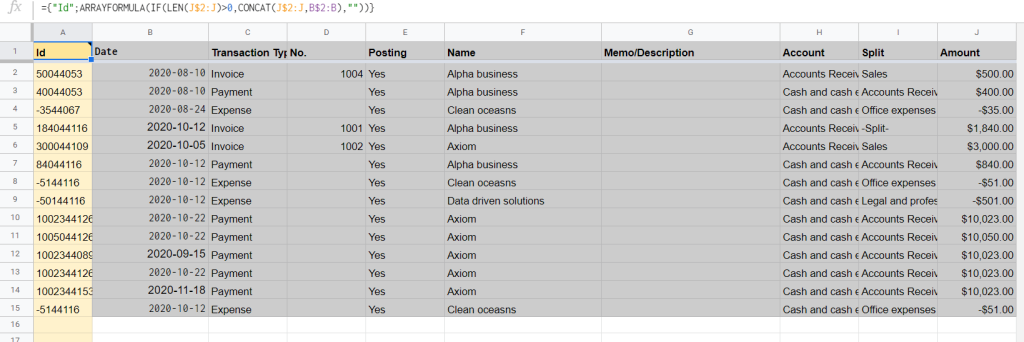
The data from HubSpot is imported to the sheet named Imported and refreshes every hour thanks to the automatic data refresh feature. The new entries automatically get their unique IDs using the following formula:
={"Id";
  ARRAYFORMULA(
    IF(
     LEN(J$2:J)>0,
     CONCAT(J$2:J,B$2:B),
     ""
    )
   )
}
In another sheet, the data is being deduplicated using the following formula:
={Imported!A1:J1;
  SORTN(
    SORT(
      FILTER(
        Imported!A2:J,
        LEN(Imported!A2:A) > 0
       ),
    1,2),
  ROWS(Imported!A2:A),
  2,1,true
  )
}
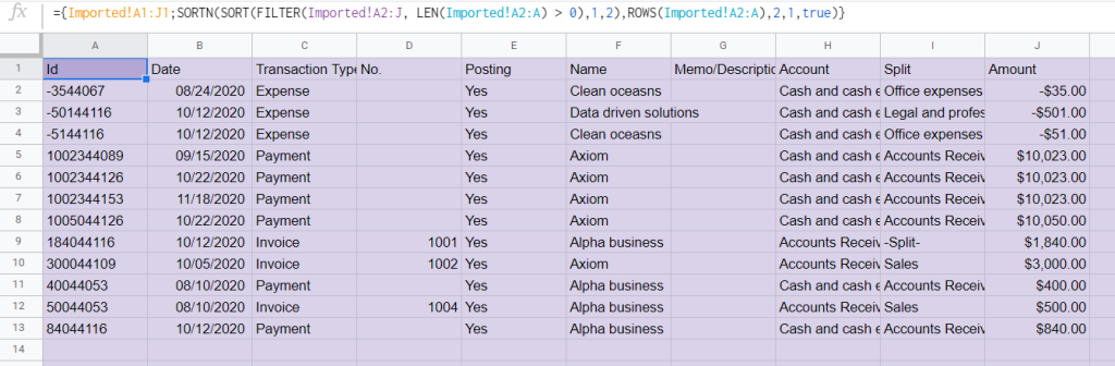
Eventually you get a refined data set that is imported from HubSpot and deduplicated absolutely automatically:
- Coupler.io ETL tool pulls data from HubSpot on a custom schedule
- Google Sheets formulas deduplicate data once it gets to the spreadsheet
The combination of these tools can provide you with astonishing integrations and automations. So, you should definitely try them out. However, we have a few more methods to cover, so keep going!
How to remove duplicates in Google Sheets using Conditional Formatting
The Conditional Formatting functionality is not actually for deleting duplicates. You can use this feature to highlight them. So, for removal, you’ll have to complete two steps:
- Identify and highlight duplicates with Conditional formatting
- Delete duplicates
Identify and highlight duplicates in Google Sheets using Conditional Formatting and the COUNTIF function
Go to the Format menu and select Conditional Formatting.
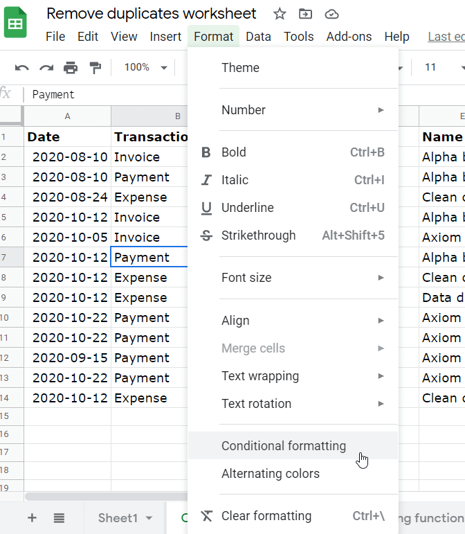
Apply the following Conditional formatting rules, depending on your goals:
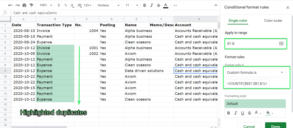
How to highlight duplicates in one column
Let’s say you want to highlight duplicates in one column. Select the column range, for example B1:B. Select “Custom formula is” as a formatting rule and apply the following COUNTIF formula:
=COUNTIF($B$1:$B1,B1)>1
Note: the values in the formula relate to the column range you choose.
And here is how it looks:
If you want to learn the logic behind this formula, check out the video “6 Ways to Highlight Duplicates in Google Sheets” by Railsware.
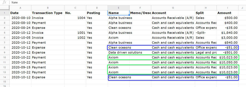
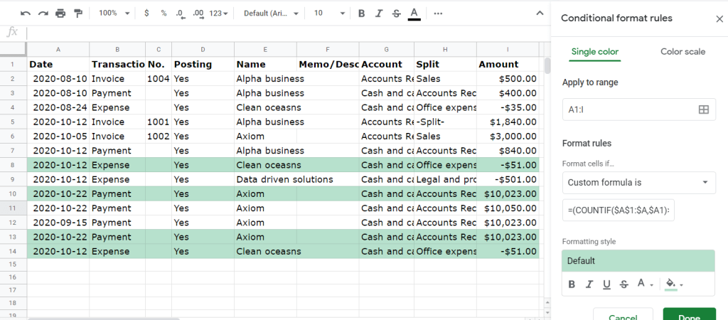
How to highlight duplicates in multiple columns
Let’s say you want to highlight duplicates in a few columns: Date (A1:A), Transaction Type (B1:B), Name (E1:E), and Amount (I1:I). Select the data range that will cover the mentioned columns, in our case – A1:I. Select “Custom formula is” as a formatting rule and apply the following COUNTIF formula:
=(COUNTIF($A$1:$A,$A1)>1)*
(COUNTIF($B$1:$B,$B1)>1)*
(COUNTIF($E$1:$E,$E1)>1)*
(COUNTIF($I$1:$I,$I1)>1)
Note: the values in the formulas are related to the columns you choose.
Duplicates on multiple conditions will be highlighted:
Remove duplicates in Google Sheets with the built-in tool
When you see the highlighted duplicates in your data set, you can easily remove them. You can do this manually or using the Remove Duplicates functionality that we described at the very beginning.
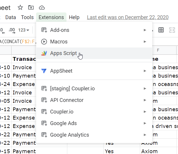
How to remove duplicates in Google Sheets using Apps Script
We had doubts as to whether we needed to include this option here, but we wanted to cover all the possible solutions. Apps Script is one of those. The idea is quite simple: you can create a custom function that will remove duplicates based on the preset conditions. It’s quite useful when you have a sheet that continuously accumulates new entries. You can specify the conditions (columns to analyze) in the function and simply run it every time you want to remove duplicates. Here is how it works:
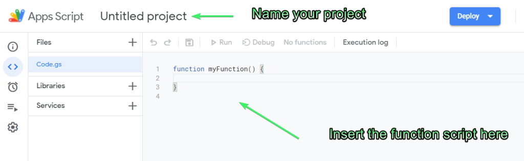
Go to the Extensions menu and select Apps Script .
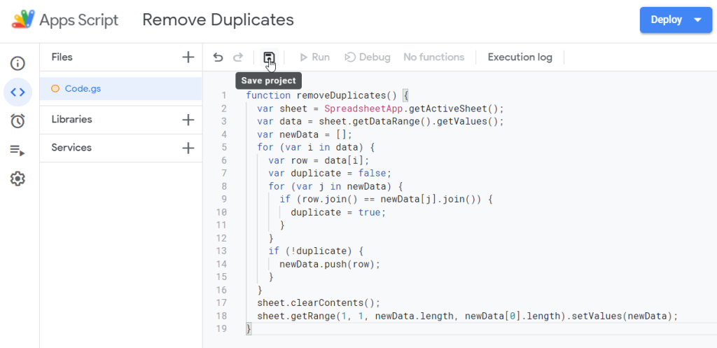
Here is the script for the basic function to remove duplicates. It analyzes all columns in the active sheet and removes duplicate rows:
function removeDuplicates() {
  var sheet = SpreadsheetApp.getActiveSheet();
  var data = sheet.getDataRange().getValues();
  var newData = [];
  for (var i in data) {
    var row = data[i];
    var duplicate = false;
    for (var j in newData) {
      if (row.join() == newData[j].join()) {
        duplicate = true;
      }
    }
    if (!duplicate) {
      newData.push(row);
    }
  }
  sheet.clearContents();
  sheet.getRange(1, 1, newData.length, newData[0].length).setValues(newData);
}
Insert it into the code block and rename your project:
Click the Save project button, then click Run next to it.
You’ll need to grant permission to access your data. Click review permissions and choose the Google account. You may get the following warning window.

Just click Advanced, and then Go to **** (unsafe).
Eventually, you’ll get back to the Apps Script editor where you’ll see that your duplicate removal function has been executed.
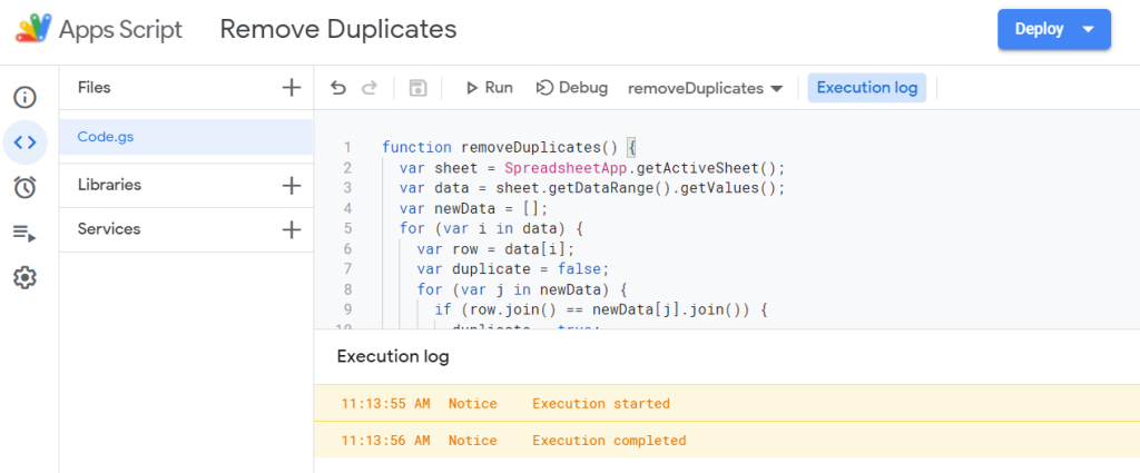
After this, it will remove duplicates in your active sheet whenever you click the Run button.
Customize the Apps Script function to remove duplicates on a specific range
The key value of using Apps Script is that you can customize it to your needs. Let’s say you want to remove duplicates on a specific range (B1:F). Here is how you need to tweak the script to make it work.
function removeDuplicates() {
var sheet = SpreadsheetApp.getActiveSheet();
var rng = sheet.getRange("B1:F")
var data = rng.getValues();
var newData = new Array();
for(i in data){
var row = data[i];
var duplicate = false;
for(j in newData){
  if(row.join() == newData[j].join()){
    duplicate = true;
  }
}
if(!duplicate){
  newData.push(row);
}
}
rng.clearContents();
sheet.getRange(1, 1, newData.length,
newData[0].length).setValues(newData);
}
For more advanced customization, you’ll need to dive deeper into the App Script specifics.
Which method to remove duplicates in Google Sheets is effective?
An attentive reader should have noticed that we did not cover how you can remove duplicates with Google Sheets add-ons. Well, this method is self-explanatory since you need to install an add-on, for example by Ablebits, and use it to highlight, combine, or remove duplicates. On the Google Workspace Marketplace, you can find a few worthy Google Sheets add-ons to do the job.
All the introduced methods are effective to remove duplicate rows but each method has its own case. The built-in functionality to remove duplicate cells works fine but it alters your original dataset. Besides, it’s manual, i.e. you will have to get rid of duplicate data every time you add new records to your spreadsheet.
If you do not want to alter the original dataset, you can create a pivot table or run a Google Sheets formula that returns the deduplicated data. This method is extremely useful for automating things, especially in combination with automated data import to Google Sheets. By the way, Apps Script can be a go here as well but it requires coding skills from your side.
As for using conditional formatting in Google Sheets to remove duplicate rows. It’s better to go this way when you need to identify and probably highlight duplicates without actually removing them since the latter will still be done manually. So, choose wisely, and good luck with your data!