You’ve probably heard about SQL, a structured query language for processing information in relational databases where the data is stored in tabular form. In spreadsheets, information is also stored in tabular form, so it would make sense to be able to query data in an SQL-like way.
Google Sheets provides this option with the help of the QUERY function. It’s very similar to SQL and it combines the capabilities of many other functions, such as FILTER, SUM, VLOOKUP, and more. So, if you already have knowledge of SQL, it will be much easier for you to master Google Sheets QUERY. If you don’t, no worries, we have put lots of effort into this article to turn it into the ultimate beginner tutorial that covers the majority of Google Sheets Query-related questions you may have.
For those of you who prefer watching to reading, we’ve created a video tutorial about the QUERY function in Google Sheets.
What is the Google Sheets Query function?
What is Query in Google Sheets? It’s a function that grabs the data based on criteria and, if necessary, amends the formatting, performs extra calculations, changes the order of columns, etc. As a result, your data source stays unchanged, and your working sheet has the selection of columns and rows that you need to complete the task.
How to use Query in Google Sheets
The Google Sheets Query function allows users to perform various data manipulations. For instance, it becomes very handy when you need to prepare data in a special format to be able to use it for building certain types of visualizations. Your data source may include too much information or be unsuitable for the specific chart formatting, or column order.
Google Sheets Query uses the Google API Query Language to retrieve and manipulate data from the Google Sheets API. For example, you want to retrieve all rows from a sheet where the value in column A is greater than 10. In this case, the mechanics of the Query function in Google Sheets will be the following:
- You create an SQL-like query using the Google API Query Language
- The function sends a request to the Google Sheets API using the query and receives the filtered data back as a result.
Google Sheets Query formula syntax
A slight spoiler at the beginning of the article – I’ll be explaining every query string separately and point to this Google Sheets spreadsheet to show how it actually works.
Now, let’s start our journey by looking at the syntax of the Google Sheets Query function.
= QUERY(data, query, [headers])
- data – a set of cells that you want to request Google Sheets to perform an inquiry on.
- query – a string that contains an inquiry composed using the Google API Query Language. Don’t forget to wrap your query into double quotation marks like this:
=query('data from Airtable'!A:L,"select *")
Or just refer to a cell with the inquiry written in the Google Query language.
- headers – an optional part of the Query formula to define the number of heading rows in your data set.
What are the literals in the Google Sheets Query function?
Literals are the various types of values you input into a spreadsheet. The following types of literals exist in the Google API Query Language:
- Strings – the text values that are put into single/double quotes. Note that they are case-sensitive. For example:
"first day" 'one person' "Burger" - Numbers – numerals used in decimal notation. For example:
1 2.5 7.15 -20.0 .8
- Date/time – this type of literal includes: 1) the word DATE and the value in the
yyyy-MM-ddformat; 2) the word TIMEOFDAY and the value in theHH:mm:ss[.SSS]format; 3) the word TIMESTAMP or DATETIME and the value in theyyyy-MM-dd HH:mm:ss[.SSS]format.
Note: every column can have only one type of literal: string or numeric (which contains numbers and date/time) values. If a given column includes more than one type of literal, then Google Sheets will pick the data type that is used more frequently for this column to execute the Query function.
How to import and query data without formulas
If you’re new to data queries or find it difficult to keep track of various Google Sheets formula syntaxes, Coupler.io offers a simpler and more intuitive solution.
You can query data from different spreadsheets and applications in real-time using Coupler.io without any formulas. This helps you save time, avoid potential errors, and have updated data.
Try it yourself for free – select the source destination in the form below and click Proceed. You can sign up with your Google account without the need to provide any payment details.
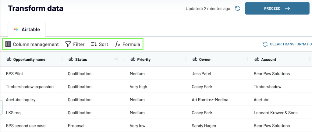
Then you’ll need to connect your data source and specify which data to import. After this, you can query and transform the data using the following options.
- Column management – hide and unhide columns as required.
- Filter – Instead of using different combinations of WHERE clauses, you can filter based on multiple criteria.
- Sort – Sort the data in ascending, descending, and by date without the ORDER BY clauses.
- Formula – create custom formulas easily using different columns.
Here is what this step looks like in the example of using Airtable to Google Sheets integration.
Now, save your transformed data in Google Sheets. Set up an automatic data refresh schedule to transfer data from Airtable to Google Sheets every 15 minutes.
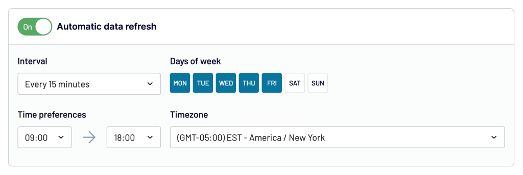
This way you’ll always have real-time queried Airtable data in Google Sheets.
Google Sheets Query clauses to design data queries
In SQL, a clause is a component of a statement that specifies a particular action.
The Google API Query Language includes 9 clauses; each of them has a unique intended purpose. They are optional, meaning that you don’t have to include all of them in one query.
One query string may contain several space-separated clauses that have to be written in this order: 1) SELECT, 2) WHERE, 3) GROUP BY, 4) PIVOT, 5) ORDER BY, 6) LIMIT, 7) OFFSET, 8) LABEL, 9) FORMAT.
Keep reading to learn more about these clauses and see the examples that accompany them. But first, let’s get some sample data to help you master your Query formula skills. We pulled a dataset from an Airtable database to Google Sheets using Coupler.io.
Now, we are ready to move on and explore the Query function with some real-life examples.
#1: Google Sheets Query: SELECT
The SELECT clause allows defining the columns you want to fetch and the order in which you want to organize them in your new worksheet. If the order is not specified, the data will be returned “as is” in a source spreadsheet.
One can use column IDs (the letters located at the top of every column in a spreadsheet), for example, SELECT A, B, or reference columns as Col1, Col2 and so on in the numerical sequence. You can also reference the results of arithmetic operators, scalar or aggregation functions as elements to order in this clause.
Note: if you are planning to embed Query into more complex formulas, we recommend referencing columns Col1, Col2, and so on in the numerical sequence. If you choose this option, then the data argument from the general Query syntax has to be enclosed in curly brackets.
= QUERY({data}, query, [headers])
Google Sheets Query SELECT all example
In our case, the ready-to-use formula will read:
=query('data from Airtable'!A:L,"select *")
'data from Airtable'!A:L– the data range to query on"select *"– select all information in the above-mentioned data set
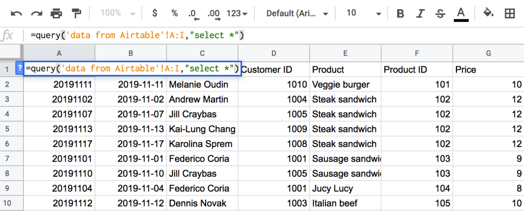
Note The headers parameter allows you to specify the number of header rows to return. If you omit the header element, the returned data will include the heading row. To remove the headers, type “0” in your Query formula like this:
=query('data from Airtable'!A:I,"select *", 0)
The same action can be carried out via Coupler.io which pulls all the data from another sheet or spreadsheet to your current document. Check out How to Reference another Spreadsheet article which explains how to set up this connection.
Google Sheets Query SELECT one or multiple columns example
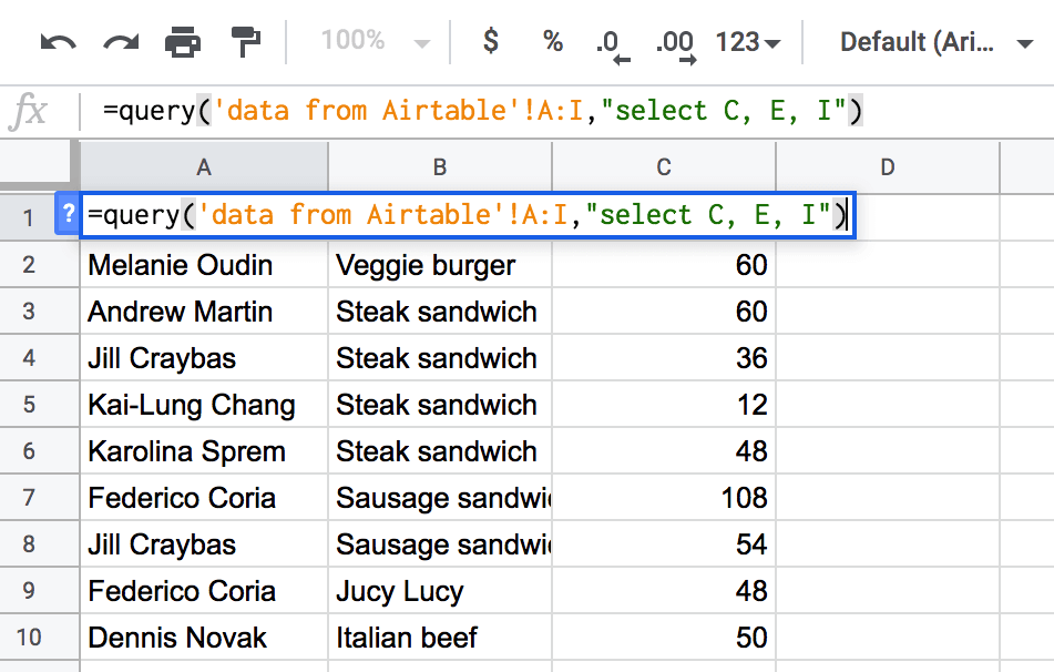
If a user wants to fetch only a certain or multiple columns, one needs to define them by a column ID like as follows:
=query('data from Airtable'!A:L,"select C, E, I")
'data from Airtable'!A:L– the data range to query on"select C, E, I"– pull all data from the columns C, E, I
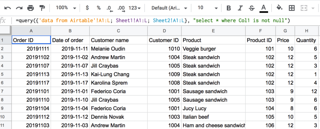
Google Sheets Query SELECT multiple sheets example
If you need to query different sheets in Google Sheets, meaning that you want to select data from several different tabs of a spreadsheet, then feel free to use the below example:
=query({'data from Airtable'!A1:L; Sheet1!A1:L; Sheet2!A1:L}, "select * where Col1 is not null")
{'data from Airtable'!A1:L; Sheet1!A1:L; Sheet2!A1:L}– an array formula enclosed into curly brackets which includes the list of sheets I want to pull data from, separated by semicolons."select * where Col1 is not null"– pull all data where the contents of the rows in column 1 (column A, Order ID) are not empty. Continue reading this article to learn more about the Where clause, as well as “is null” and “is not null” operators.
Note: if you want to query some data from another spreadsheet, then I would recommend you use a combination of QUERY and IMPORTRANGE.
#2: Google Sheets Query WHERE
Users apply WHERE when they need to pull specific rows from the columns, they have already identified in the SELECT clause, which satisfies one or more conditions.
To compare values across rows, one needs to be aware of these basic logical operators that accompany the WHERE clause.
| Operator | Meaning |
|---|---|
| <= | Less than or equal |
| < | Less than |
| > | More than |
| >= | More than or equal |
| = | Equal |
| != or <> | Not equal |
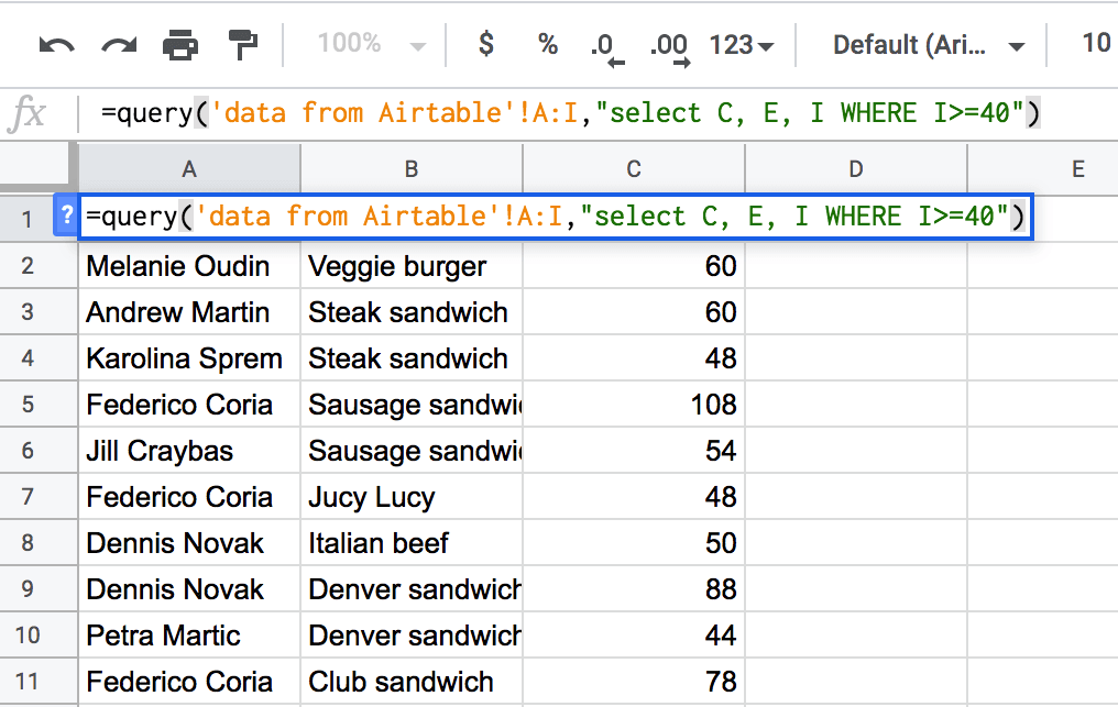
Google Sheets Query WHERE basic operators example
In my case, the ready-to-use formula will read:
=query('data from Airtable'!A:L,"select C, E, I WHERE I>=40")
'data from Airtable'!A:L– the data range to query on"select C, E, I WHERE I>=40"– pull the data from columns C, E, I, where the value in column I (total price) is more than or equals 40.
Note: if you want to say that the cell is empty or its contents equal 0 – use the is null operator, and if you want to select rows that are not empty, then enter is not null.
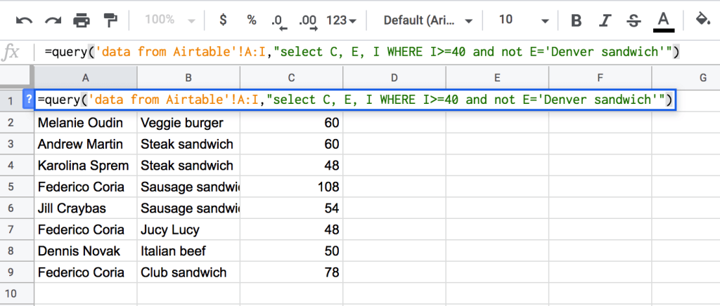
Google Sheets Query WHERE combined conditions example
One can combine several conditions using and, or, and not as part of the WHERE clause in the query like this:
=query('data from Airtable'!A:L,"select C, E, I WHERE I>=40 and not E='Denver sandwich'")
'data from Airtable'!A:L– the data range to query on"select C, E, I WHERE I>=40 and not E='Denver sandwich'"– pull the data from columns C, E, I, where the value in column I (total price) is more than or equals 40 and where the string in column E (product) does not include the Denver sandwich.
Google Sheets Query WHERE advanced operators example
Use these advanced comparison operators to run more complex queries:
| Operator | Meaning |
| starts with | Compares the value with the condition and searches for full correspondence in the prefix or at the beginning of the string. |
| ends with | Compares the value with the condition and searches for full correspondence in the suffix or at the end of the string. |
| contains | Compares the value with the condition and searches for its presence in any part of the string (be it at the beginning, in the middle, or at the end of the argument). |
| matches | This match is performed via the usage of regular expressions enclosed in single quotation marks. |
| like | Compares the value with the condition expressed by the usage of two arguments: 1) % – is used when there may be either no characters, one or multiple ones of any type and kind; 2) _ (underscore) – is used when there can be only one single character of any kind. |
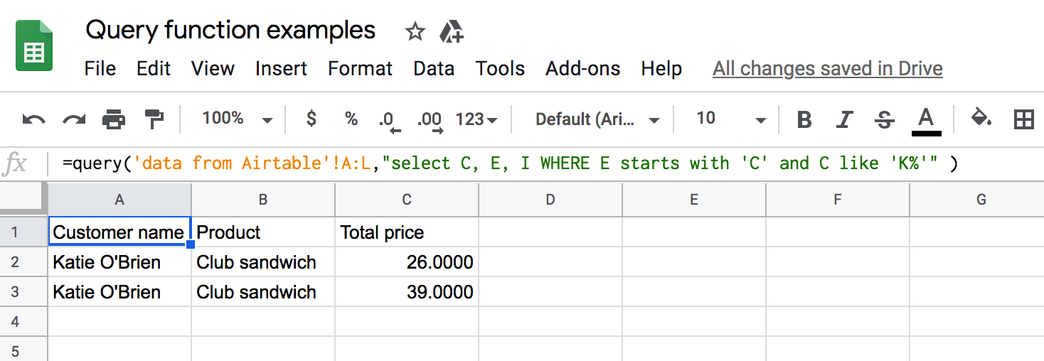
In my case, the ready-to-use formula will read
=query('data from Airtable'!A:L,"select C, E, I WHERE E starts with 'C' and C like 'K%'")
'data from Airtable'!A:L– the data range to query on"select C, E, I WHERE E starts with 'C' and C like 'K%'"– the string pulls the data from columns C, E, I, where the value in column E (product) starts with the “C” letter and where the string in column C (customer name) starts with the “K” letter.
Google Sheets Query Matches example
The matches operator helps in advanced pattern matching using regular expressions and use complex search criteria within queries.
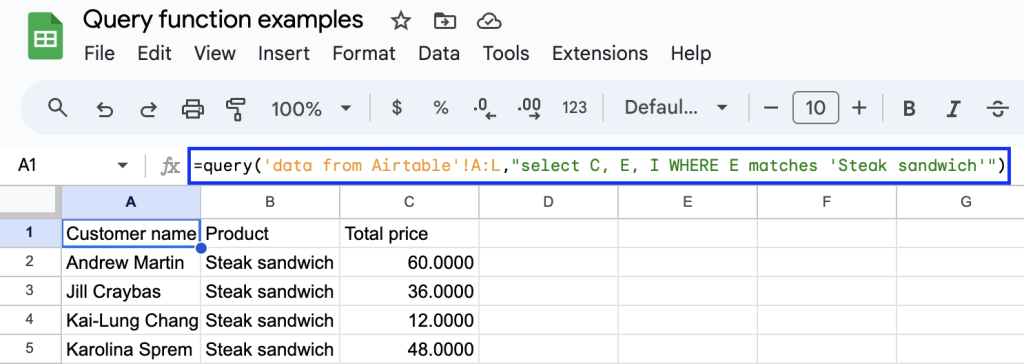
=query('data from Airtable'!A:L,"select C, E, I WHERE E matches 'Steak sandwich'")
'data from Airtable'!A:I– the data range to query on"select C, E, I "select C, E, I WHERE E matches 'Steak sandwich'"– filters the dataset to return only the rows where column E (product) exactly matches the phrase “Steak sandwich”. It then displays the C (customer name), E (product), and I (total price) columns for those filtered rows.
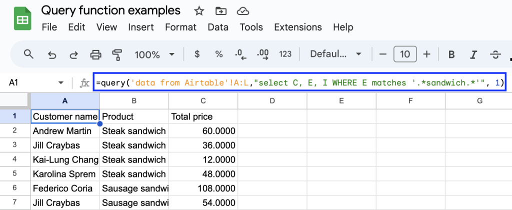
Alternatively, if you want to filter the data based on a partial match, use regular expressions (RegEx) in the formula.
=query('data from Airtable'!A:L,"select C, E, I WHERE E matches '.*sandwich.*'", 1))
'data from Airtable'!A:I– query data"select C, E, I "select C, E, I WHERE E matches '.*sandwich.*'"– filters the dataset to return only the rows where column E (product) partially matches the phrase “sandwich”. Use regular expressions like ‘.*’ before and after “sandwich” to match any characters that occur before or after “sandwich”.
#3: Google Sheets Query GROUP BY
This GROUP BY clause is used to group values across the selected data range by a certain condition.
Note: the columns that you mention in the SELECT clause must be present in either the GROUP BY clause or as part of the aggregation function (e.g. avg, count, max, min, sum).
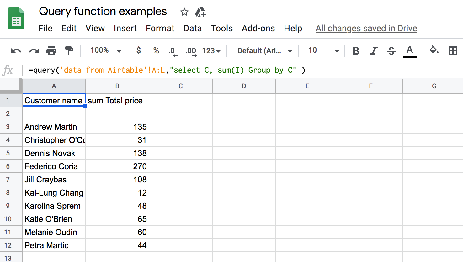
Example of GROUP BY one column: Google Sheets Query SUM
In my case, the ready-to-use formula will read:
=query('data from Airtable'!A:L,"select C, sum(I) Group by C")
'data from Airtable'!A:L– the data range to query on"select C, sum(I) Group by C"– the string sums purchases (column I) and groups them by customer names (column C).
Example of Google Sheets Query GROUP BY multiple columns
In my case, the ready-to-use Google Sheets Query GROUP By multiple columns formula will read:
=query('data from Airtable'!A:L,"select C, H, sum(I) Group by C,H")
'data from Airtable'!A:L– the data range to query on"select C, H, sum(I) Group by C,H"– the string pulls the data from columns C and H, sums purchases (column I), and groups data by customer names (column C).
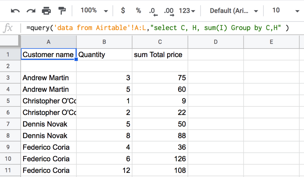
Note: when using this formula, specify all columns that you defined in the Select clause in the Group by clause as well. The output will be grouped by the first column ID mentioned in the Group by clause.
#4: Google Sheets Query PIVOT
Using the PIVOT clause one can convert rows into columns, and vice versa, as well as aggregate, transform, and group data by any field.
Note: the columns that you mention in the SELECT clause must be present in either the GROUP BY clause or as part of the aggregation function (e.g. avg, count, max, min, sum).
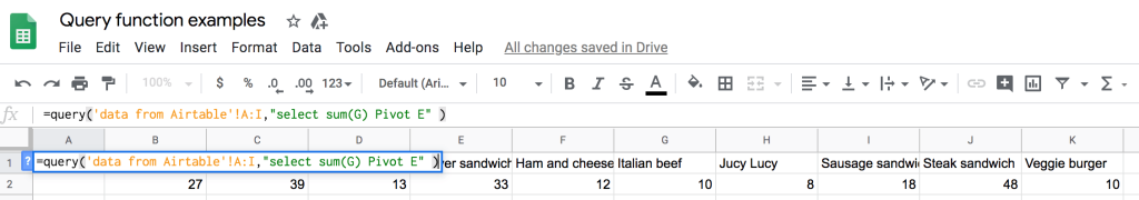
Google Sheets Query PIVOT without GROUP BY example
If rows of the pivot columns contain the same values, the PIVOT clause will aggregate them. So, if you don’t use GROUP BY as part of the PIVOT clause, as a result, you will get a table with one row only.
=query('data from Airtable'!A:L,"select sum(G) Pivot E")
'data from Airtable'!A:L– the data range to query on"select sum(G) Pivot E"– the string sums the prices of all burgers sold (column G) and groups them by the product (column E).
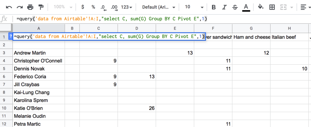
Google Sheets Query PIVOT with GROUP BY example
In my case, the ready-to-use formula will read:
=query('data from Airtable'!A:L,"select C, sum(G) Group BY C Pivot E",1)
'data from Airtable'!A:L– the data range to query on"select C, sum(G) Group BY C Pivot E"– the string returns a PIVOT table which has the names of burgers (column E) in the heading row, and the list of customers (column C) as the main column, showing which burgers customers bought and how much they paid (column G).
#5: Google Sheets Query ORDER BY (ascending or descending)
In Google Sheets, you can sort data using different functions including SORT, SORTN, or QUERY. Within Google Sheets QUERY, you can sort data across columns in ascending (ASC) or descending (DESC) order using the ORDER BY clause.
The elements to order within the ORDER BY clause can be column IDs or the results of arithmetic operators, scalar, or aggregation functions.
Example of Google Sheets Query ORDER BY to sort in ascending order
In my case, the ready-to-use formula will read:
=query('data from Airtable'!A:L,"select * where A is not null order by A")
'data from Airtable'!A:L– the data range to query on"select * where A is not null order by A"– the string pulls all data and orders it by order ID (column A) in ascending order.
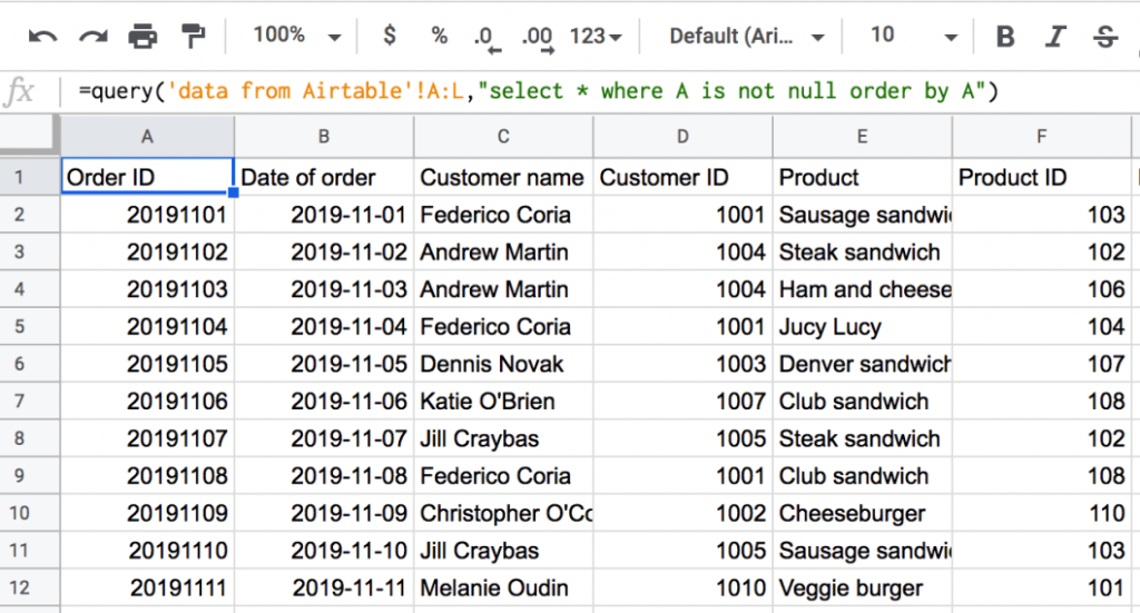
Note: it is crucial to add is not null to the string to make sure the output does not account for empty cells and bring them all up in your table.
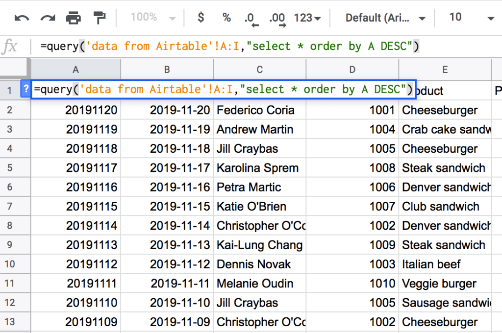
Example of Google Sheets Query ORDER BY to sort in descending order
If rows of the pivot columns contain the same values, the PIVOT clause will aggregate them. So, if you don’t use GROUP BY as part of the PIVOT clause, you will get a table with one row only.
In my case, the ready-to-use formula will read:
=query('data from Airtable'!A:I=L,"select * order by A DESC")
'data from Airtable'!A:L– the data range to query on"select * order by A DESC"– the string pulls all data and orders it by order ID (column A) in descending order.
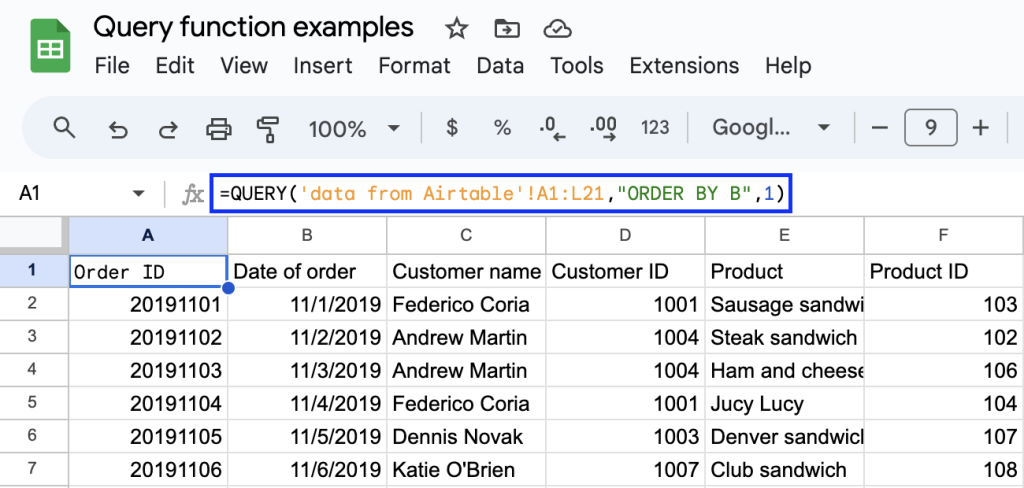
Example of Google Sheets Query Sort By Date
To sort the data by date, you can use the ORDER BY clause followed by date.
=QUERY('data from Airtable'!A1:L21,"ORDER BY B",1)
'data from Airtable'!A:I– the query data range"ORDER BY B"– the string to sort the entire dataset based on the values in column B (date of order) in ascending order.
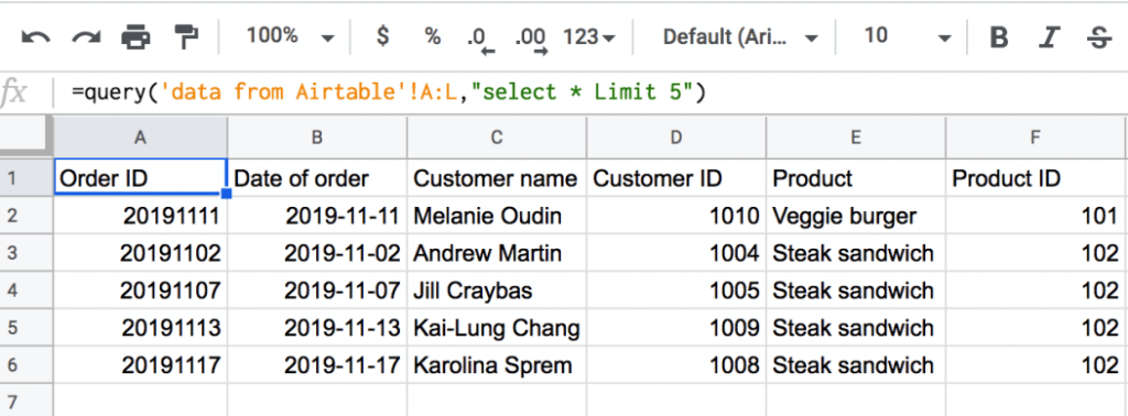
#6: Google Sheets Query LIMIT (+ formula example)
The LIMIT clause reduces the number of rows pulled from another sheet.
In my case, the ready-to-use formula will read:
=query('data from Airtable'!A:L,"select * Limit 5")
'data from Airtable'!A:L– the data range to query on- “
select * Limit 5"– the string pulls all data and limits the returned result to the first 5 rows + the header.
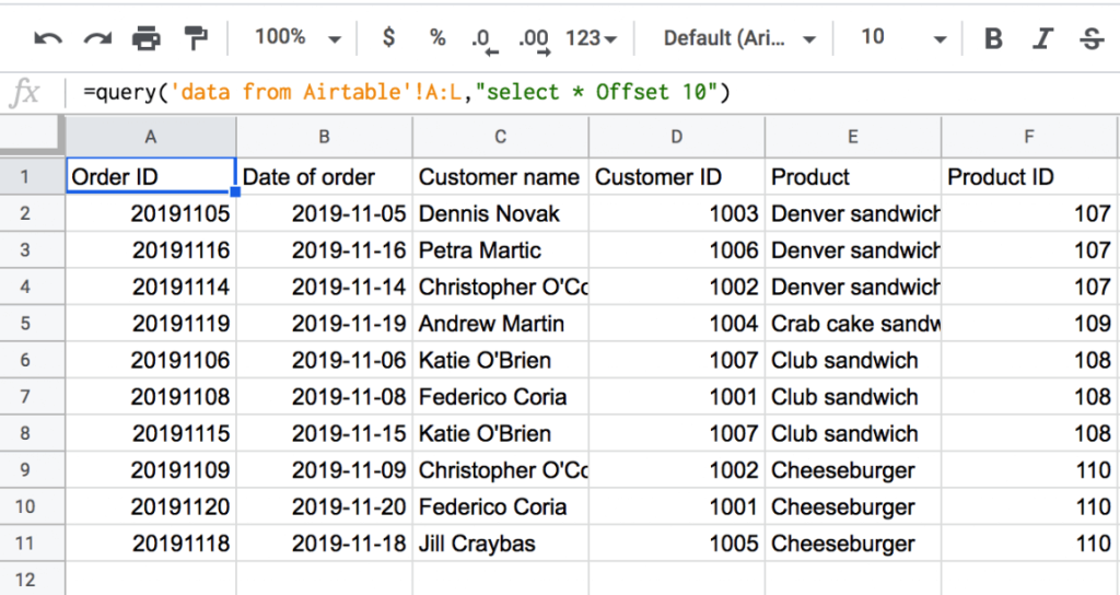
#7: Google Sheets Query OFFSET
Using this clause you may ask Google Sheets to skip a pre-defined number of rows from the top of your data source spreadsheet.
Google Sheets Query OFFSET only formula example
In my case, the ready-to-use formula will read:
=query('data from Airtable'!A:L,"select * Offset 10")
'data from Airtable'!A:L– the data range to query on"select * Offset 10"– the string pulls all data and skips the first 10 rows excluding the header.
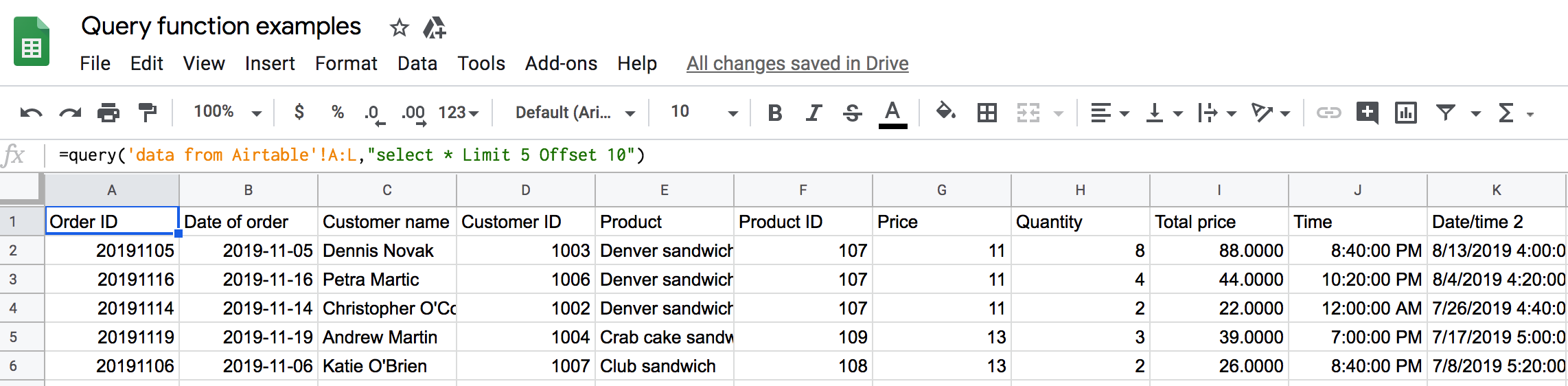
Google Sheets Query OFFSET accompanied by LIMIT example
If OFFSET is combined with the LIMIT clause, though it follows LIMIT in the syntax, it will apply first.
In my case, the ready-to-use formula will read:
=query('data from Airtable'!A:L,"select * Limit 5 Offset 10")
'data from Airtable'!A:L– the data range to query on"select * Limit 5 Offset 10"– the string pulls all data, skips the first 10 rows, and limits the result to 5 rows excluding the header.
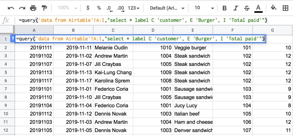
#8: Google Sheets Query LABEL (+formula example)
The LABEL clause allows you to assign a name to a heading field of one or multiple columns. However, you won’t be able to apply it instead of a column ID in a query string.
One can use column IDs or the results of arithmetic operators, scalar, or aggregation functions as elements in this clause.
In my case, the ready-to-use formula will read:
=query('data from Airtable'!A:L,"select * label C 'customer', E 'Burger', I 'Total paid'")
'data from Airtable'!A:L– the data range to query on"select * label C 'customer', E 'Burger', I 'Total paid'"– the string pulls all data, and gives columns C, E and I new labels.
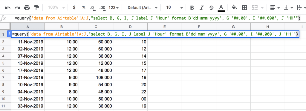
#9: Google Sheets Query FORMAT
Users apply the FORMAT clause to format NUMBER, DATE, TIME, TIMEOFDATE, and DATETIME values for one or multiple columns.
Example of FORMAT clause: Google Sheet Query Date
In my case, the ready-to-use formula will read:
=query('data from Airtable'!A:L,"select B, G, I, J label J 'Hour' format B 'dd-mmm-yyyy', G '##.00', I '##.000', J 'HH'")
'data from Airtable'!A:L– the data range to query on"select B, G, I, J label J 'Hour' format B 'dd-mmm-yyyy', G '##.00', I '##.000', J 'HH'"– the string pulls the data from columns B, G, I, and J, formats the date in the B column, the number in the G and I columns, and the time in the J column, also changing its label to ‘Hours’.
Data manipulation with Google Sheets Query
The Google Visualization API query language specifies the three core functions and operators that are called to help you manipulate your data:
- Arithmetic operators
- Aggregation functions
- Scalar functions
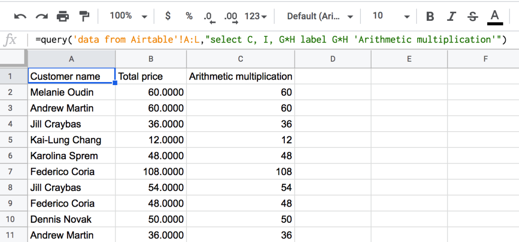
Google Sheets Query arithmetic operators (+ formula example)
Arithmetic operators help users execute basic calculations. They include + (plus), - (minus), / (divide), * (multiply), where the parameters are two numbers and the result the Query function returns is a number as well.
In my case, the ready-to-use formula will read:
=query('data from Airtable'!A:L,"select C, I, G*H label G*H 'Arithmetic multiplication'")
'data from Airtable'!A:L– the data range to query on"select C, I, G*H label G*H 'Arithmetic multiplication'"– the string pulls the data from columns C, I, multiplies the value in column G by the number in column H, and changes the label of the column with multiplication to ‘Arithmetic multiplication’.- Note, that the pulled from the data source sheet value in column B equals the calculated result shown in column C.
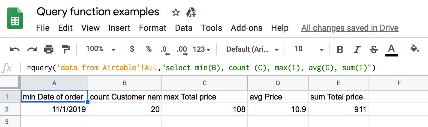
Google Sheets Query aggregation functions (+ formula example)
Aggregation functions apply to one column ID and execute an operation across data in all rows of this specific column. Usually, aggregation functions appear in the SELECT, ORDER BY, LABEL, and FORMAT clauses. Additionally, they also may refer to a data set formed as part of the PIVOT or GROUP BY clauses.
Note: they cannot be used as part of these clauses: WHERE, GROUP BY, PIVOT, LIMIT, or OFFSET.
The aggregation functions include the following categories:
| Supported number as a column type and the result is a number as well. | avg() – provides the average of all numbers in a column.sum() – provides the sum of all numbers in a column. |
| Support any column type and the result is a number. | count() – provides the quantity of items in a column (rows with empty cells are not calculated). |
| Support any column type and the result is going to be the same as the column type. In this case, earlier dates will be lesser than the later ones; and the text values are lined up alphabetically, where case-sensitivity is considered as well. | max() – provides the maximum value of all in a column.min() – provides the minimum value of all in a column. |
In my case, the ready-to-use formula will read:
=query('data from Airtable'!A:L,"select min(B), count (C), max(I), avg(G), sum(I)")
'data from Airtable'!A:L– the data range to query on"select min(B), count (C), max(I), avg(G), sum(I)"– the string fetches the minimum value from the B column, counts the number of items in the C column, pulls the maximum value from I column, calculates the average of the G column contents, and sums up the numbers in the I column.
Google Sheets Query scalar functions (+ formula example)
Scalar functions are used to convert a given parameter into another value.
Note: if you use one of the Scalar functions, the heading cell of the column will be amended.
One may use these functions as part of the SELECT, WHERE, GROUP BY, PIVOT, ORDER BY, LABEL, and FORMAT clauses.
Below I have split the functions into groups by the required parameters and the types of values they return.
DATE or DATETIME scalar functions
Scalar functions that support a single parameter of type DATE or DATETIME and return a number as a result:
| Function name | What it does |
| year() | Fetches the year from a DATETIME/TIMESTAMP or DATE value. |
| month() | Fetches the month from a DATETIME/TIMESTAMP or DATE value on a scale from 0 to 11, where January equals 0, February is 1, and so on finishing with December being 11. |
| day() | Fetches the day of the month from a DATETIME/TIMESTAMP or DATE value. |
| quarter() | Fetches the quarter from a DATETIME/TIMESTAMP or DATE value on a scale from 1 to 4, where 1 corresponds to the first quarter, 2 to the second, and so on. |
| dayOfWeek() | Fetches the day of the week from a DATETIME/TIMESTAMP or DATE value on a scale from 1 to 7, where 1 corresponds to Sunday, 2 to Monday, and so on. |
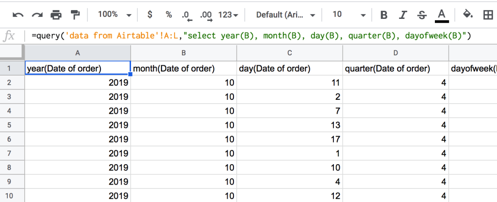
In my case, the ready-to-use formula will read:
=query('data from Airtable'!A:L,"select year(B), month(B), day(B), quarter(B), dayofweek(B)")
'data from Airtable'!A:L– the data range to query on"select year(B), month(B), day(B), quarter(B), dayofweek(B)"– the string fetches the year, month, day, quarter, and day of the week from the B column (date of order).
DATETIME or TIMEOFDAY scalar functions
Scalar functions that support a single parameter of type DATETIME or TIMEOFDAY and the result is a number:
| Function name | What it does |
| hour() | Fetches the hour from a DATETIME/TIMESTAMP or DATE value. |
| minute() | Fetches the minute from a DATETIME/TIMESTAMP or DATE value. |
| second() | Fetches the second from a DATETIME/TIMESTAMP or DATE value. |
| millisecond() | Fetches the millisecond of the week from a TIMEOFDAY or DATETIME/TIMESTAMP value. |
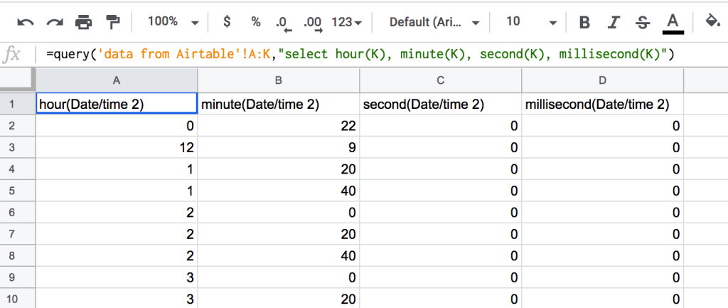
In my case, the ready-to-use formula will read:
=query('data from Airtable'!A:K,"select hour(K), minute(K), second(K), millisecond(K)")
'data from Airtable'!A:K– the data range to query on"select hour(K), minute(K), second(K), millisecond(K)"– the string fetches the hour, minute, second, and millisecond from the K column (date/time 2).
Scalar functions to make upper or lower case values
Scalar functions that support a single parameter of type String and the result is a String as well:
| Function name | What it does |
| upper() | Converts the string value by replacing all letters with the uppercase ones. |
| lower() | Converts the string value by replacing all letters with the lowercase ones. |
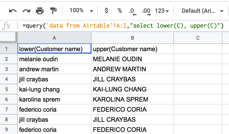
In my case, the ready-to-use formula will read:
=query('data from Airtable'!A:I,"select lower(C), upper(C)")
'data from Airtable'!A:I– the data range to query on"select lower(C), upper(C)"– the string fetches data from the C column (customer name) and converts all information to lower and upper cases.
Scalar function to calculate the date difference
A scalar function that supports two parameters of type DATE or DATETIME (can be any one of these two) and the result is a number:
| Function name | Calculates the difference between the two DATE / DATETIME / TIMESTAMP values and displays the result as a number of days. Please note that the time value is not taken into consideration during the calculation. |
| dateDiff() | Calculates the difference between the two DATE / DATETIME / TIMESTAMP values and displays the result as a number of days. Please note that time value is not taken into consideration during the calculation. |
Calculation of the difference between two dates example
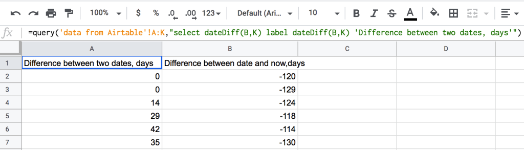
In my case, the ready-to-use formula will read:
=query('data from Airtable'!A:K,"select dateDiff(B,K) label dateDiff(B,K) 'Difference between two dates, days'")
'data from Airtable'!A:K– the data range to query on"select dateDiff(B,K) label dateDiff(B,K) 'Difference between two dates, days'"– the query string calculates the difference in days between the dates in columns B and K (B-K) and changes the label of the column respectively.
Calculation of the difference between date and now example
In order to calculate the difference between a given date and the present time, we will need to familiarize ourselves with the now() function first.
It does not require any parameter and returns a DATETIME as a result:
| Function name | Meaning |
| now() | Displays the current DATETIME value using the GMT time. |
The ready-to-use formula computing the difference is as follows:
=query('data from Airtable'!A:K,"select dateDiff(B,now()) label dateDiff(B,now()) 'Difference between date and now,days'")
'data from Airtable'!A:K– the data range to query on"select dateDiff(B,now()) label dateDiff(B,now()) 'Difference between date and now,days'"– the query string calculates the difference in days between the date in column B and now (current date and time) and changes the label of the column respectively.
Scalar function to convert values into a date
This function supports one of the parameters at a time: a DATE, DATETIME, or a NUMBER and returns a DATE:
| Function name | What it does |
| toDate() | Converts a DATE, DATETIME, or a NUMBER value into a DATE: – If a given parameter is a DATE, the returned value will be the same DATE value – If a given parameter is a DATETIME, the returned value will be the DATE only – If a given parameter is a NUMBER, the returned value will be the DATE calculated as the number of milliseconds after 01.01.1970 00:00:00 GMT (the Epoch). |
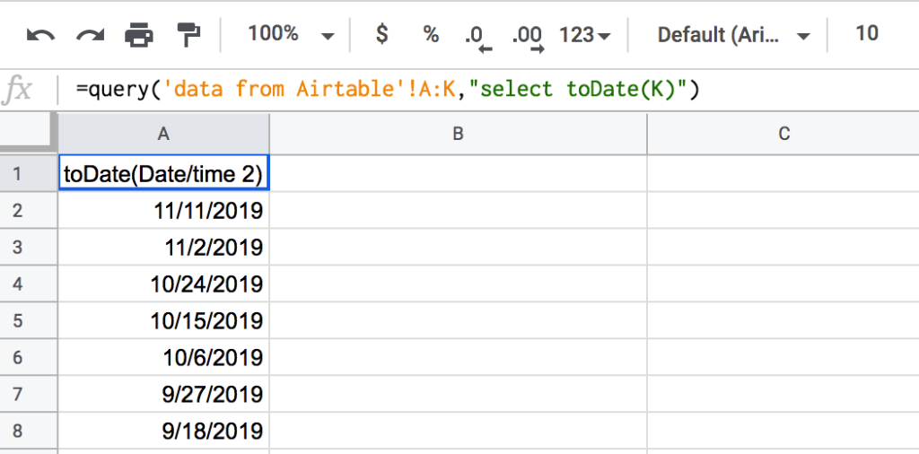
In my case, the ready-to-use formula will read:
=query('data from Airtable'!A:K,"select toDate(K)")
'data from Airtable'!A:K– the data range to query on"select toDate(K)"– the query string returns the date value from the DATETIME parameter.
Query in Google Sheets to start your path with SQL
The Google Sheets Query function helps manage data across spreadsheets for various use cases. Understanding the different Query syntax with examples will lay a strong foundation to query data in other data warehouses like BigQuery. But memorizing all the clauses and how to wrap them in formulas can be a challenge, along with the frequent errors from Google.
Coupler.io is an alternate solution to import and query real-time data easily. Not just spreadsheets, it can query data from multiple sources without any formulas. Coupler.io replaces a lot of complex Google Sheets Query formulas like WHERE and ORDER BY with simple features like column management, sort, filter, and custom columns.

Automate data export with Coupler.io
Get started for free