Oftentimes, you’ll need to merge cells in Google Sheets, either to combine some information or change the look of a spreadsheet. There are various approaches to the task that can produce different outcomes, and what will work best depends on your individual needs.
We’ll discuss each available approach and demonstrate them one by one with an example data set. Let’s get to it, then!
How to merge cells in Google Sheets
There are roughly two ways to merge cells in Google Sheets:
- With a button or menu items available in the Google Sheets interface
- With a relevant function or operator
Why overcomplicate things with functions, though? Well, here’s a trick – merging data with the default options doesn’t preserve all the data in cells. To understand this limitation, let’s look at a simple example.
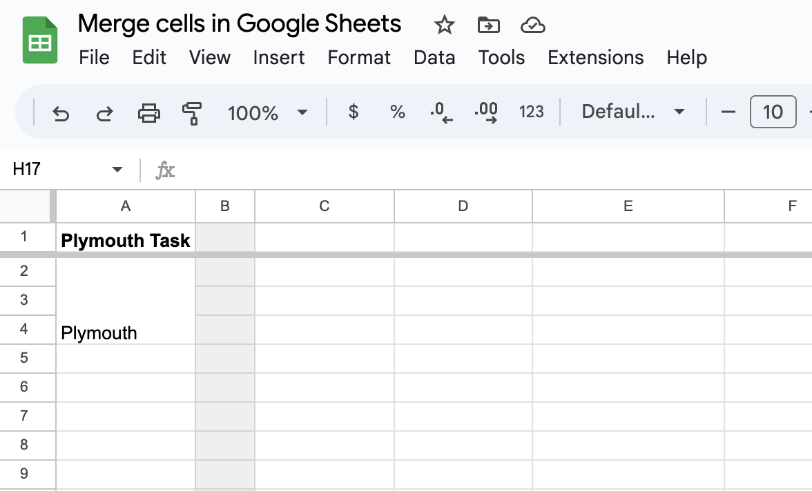
Let’s say you have a spreadsheet with three cells:
- A2 with “
Plymouth“ - A3 with “
Road Runner“ - A4 with “
1970“
You want to combine all three cells into a single cell. The most natural thing is to highlight the cells and click the “merge cells” button in the menu, optionally selecting the type of merge.

You can see the same options if you venture to the Format menu on top:

Whichever way you choose to merge cells in Google Sheets, you may see a popup informing you that some data will be lost. In fact, only the top-leftmost value will be preserved, which is precisely what happens.
So this approach clearly won’t work if you care about preserving all data. However, if the cells are empty, or you only care about the top-leftmost value, you can rely on either of these methods. For example, let’s merge cells in columns D to H:
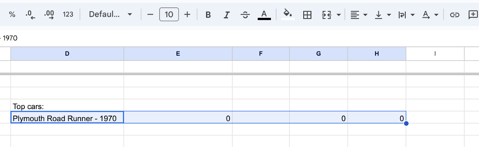
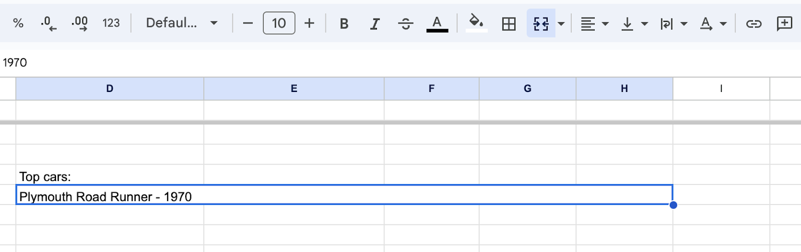
Here’s the outcome:
Shortcut to merge cells in Google Sheets
While there’s no direct Google Sheets shortcut to merge data, you can use a handy shortcut to jump to the relevant menu and confirm your choice then. Here’s how to do it:
- Select the cells you want to merge
- Open the Format menu by pressing;
- On Windows: Alt+0
- On Mac: Ctrl+Option+O
- Press M to enter the Merge cells menu
- If Merge all works for you, you can press ENTER to select it. Otherwise, simply use a cursor to choose the right option.

Connect and merge your data with Coupler.io
Get started for freeHow to merge cells in Google Sheets without losing data
In most cases, however, you will want to preserve all data that you merge. To do that, you’ll need to use the relevant functions or operators that will combine all data and insert the result into a new cell. One way to do this is with an & operator that merges values from the chosen cells, for example:

The outcome isn’t ideal yet because we didn’t add the needed delimiters, but you should get the idea.

Once you merge all the required cells in the dataset, you can overwrite an existing cell with the merged data, as in paste the contents of cell A6 into A2 and delete what still remains in A3 and A4. Be sure, however, to paste values only, as otherwise, you’ll break the formula.

We’ll discuss an & operator more in the following chapters. We’ll also talk about five functions that can perhaps offer a more elegant outcome or be more convenient when trying to merge more complex datasets:
- CONCAT
- CONCATENATE
- JOIN
- TEXTJOIN
- SUBSTITUTE
Formula to merge cells in Google Sheets
We’ll continue with our automotive example, but we not only want to merge data but also make it readable and properly formatted. As a reminder, we have 3 cells:
- A2 with “
Plymouth“ - A3 with “
Road Runner“ - A4 with “
1970“
In a separate cell, we want to merge them and get the following outcome: “Plymouth Road Runner – 1970”.
Let’s start with a comparison table that will share different aspects of the formulas/operations we’re going to use:
| Can add delimiter(s) | Merging more than 2 cells | Merging date and time | Formula syntax | |
| & | Yes | Yes | Only when combined with the TEXT function | =cell#1&"delimiter"&cell#2&... |
| CONCAT | No | No | Only when combined with the TEXT function | =concat(cell#1, cell#2) |
| CONCATENATE | Yes | Yes | Only when combined with the TEXT function | =concatenate(data_string#1,"delimiter",data_string#2…) |
| JOIN | Yes | Yes | Yes | =join("delimiter",array#1,array#2…) |
| TEXTJOIN | Yes | Yes | Yes | =textjoin("delimiter",ignore-empty,array#1,array#2…) |
| SUBSTITUTE | Yes | Yes | Yes | =substitute("merge_pattern","text_to_search_for", "cell_to_replace_with", [occurrence_number]) |
& (ampersand) operator
The ampersand (&) is a concatenation operator that can be used to merge cells in Google Sheets. It also allows you to use different delimiters to separate the concatenated values.
Syntax
Without delimiters
=cell#1&cell#2&cell#3...
With delimiters
=cell#1&"delimiter"&cell#2&"delimiter"&cell#3&...
Plymouth task
Let’s apply the following formula to merge the cells for our Plymouth task:
=A2&" "&A3&" - "&A4
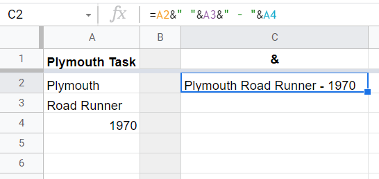
Ampersand did the job! However, this option might not be very convenient if you need to merge a really large number of cells. So, let’s keep going.
CONCAT function
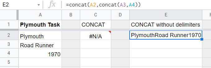
CONCAT is a function that concatenates data which is precisely what we want to do. However, the limitation of CONCAT is that it can combine only two cells at a time. But even that can be overcome with a workaround! Let’s talk first about standard usage.
Syntax
=concat(cell#1, cell#2)
Plymouth task
We need to merge three cells within the Plymouth task, which means the CONCAT is a no-go. If you use the following formula
=concat(A2,A3,A4)
it will return
#N/A error Wrong number of arguments to CONCAT. Expected 2 arguments, but got 3 arguments.

However, a workaround exists:
=concat(A2,concat(A3,A4))
This formula will merge three values without a delimiter.
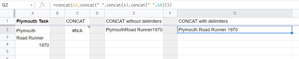
Put in a bit more effort, and here is a formula with delimiters:
=concat(A2,concat(" ",concat(A3,concat(" ",A4))))
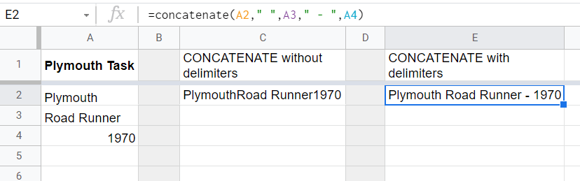
CONCATENATE function
CONCATENATE, unlike CONCAT, can accept any number of cells or even an entire data range which makes handling our task possible without workarounds.
Syntax
Without delimiters
=concatenate(data_range)
With delimiters
=concatenate(data_string#1,"delimiter",data_string#2,"delimiter",data_string#3...)
Plymouth task
Let’s use the CONCATENATE function to merge cells within the Plymouth task. We’ll apply two formulas, with and without delimiters:
=concatenate(A2," ",A3," - ",A4)
and
=concatenate(A2:A4)
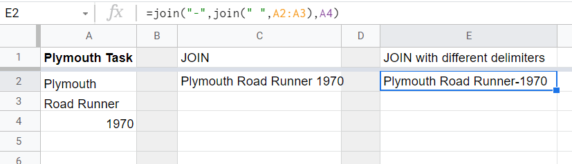
JOIN function
JOIN is a function to concatenate values in one or several one-dimensional arrays (rows or columns) using a specified delimiter.
Syntax
=join("delimiter",array#1,array#2,array#3…)
Plymouth task
At first sight, JOIN does not let you apply different delimiters as CONCATENATE or &:
=join(" ",A2:A4)
However, a bit of creativity and you can handle this. Here is a JOIN formula to specify different delimiters:
=join("-",join(" ",A2:A3),A4)
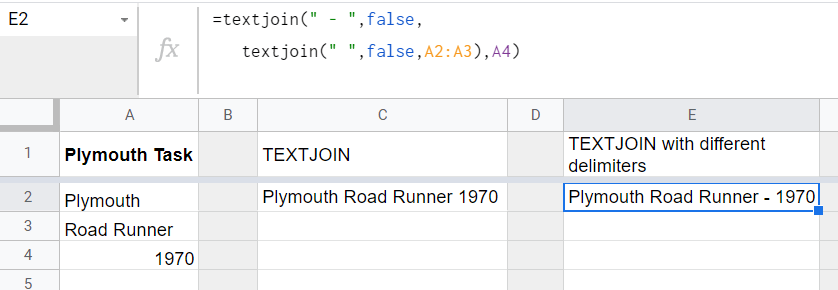
TEXTJOIN function
TEXTJOIN is a function to concatenate text values in one or several one-dimensional arrays (rows or columns) using a specified delimiter. Simply: JOIN for text values only.
Syntax
=textjoin("delimiter",ignore-empty,array#1,array#2,array#3…)
ignore-empty– if false, each empty cell within the array will be added as a delimiter; if true, empty cells will be ignored.
Plymouth task
We have only text values in our Plymouth task, so the TEXTJOIN formula will handle it.
=textjoin(" ",false,A2:A4)
And here is a TEXTJOIN formula to use different delimiters for merged cells:
=textjoin(" - ",false, textjoin(" ",false,A2:A3),A4)
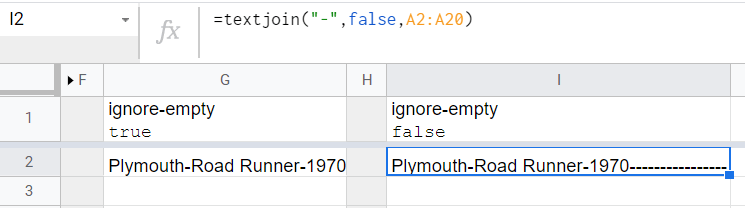
How ignore-empty works
Let’s increase the array we use within the Plymouth task up to A20 cell and change the delimiter to “-“. Check out the results returned with the ignore-empty parameter set as either true
=textjoin("-",true,A2:A20)
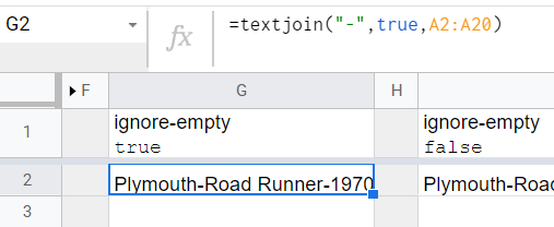
or false
=textjoin("-",false,A2:A20)
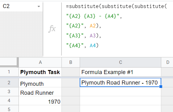
BONUS: SUBSTITUTE function
You may know SUBSTITUTE – a Google Sheets function to replace existing text strings with new ones. At the same time, it can serve as a way to merge cells (and even columns). Data analysts from Railsware actively use this approach in their workflows.
SUBSTITUTE formula syntax for merging cells:
=substitute("merge_pattern","text_to_search_for", "cell_to_replace_with", [occurrence_number])
merge_pattern– specify the order of cells and delimiters to merge. For example, A2-A3:A4.
Note: It’s not necessary to use cell indexes in the merge_pattern. You’re free to specify any text, which then will be replaced with a corresponding cell value.
text_to_search_for– specify the text from the merge_pattern to be replaced.cell_to_replace_with– specify the cell, which will replace text_to_search_for.[occurrence_number]– an optional parameter to specify the number of text_to_search_for instances to replace. By default, all instances will be replaced.
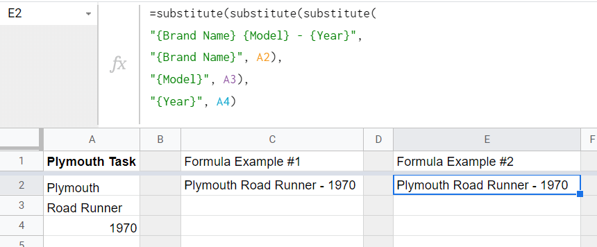
Plymouth task
According to the task, we’re merging three cells (A2, A3, A4) with two delimiters (” “, ” – “). So, the merge_pattern is the following: A2 A3 – A4. Now, we need to assign a cell index to each text_to_search_for instance to implement the replacement. Here is how the formula will look:
=substitute(substitute(substitute("{A2} {A3} - {A4}","{A2}", A2),"{A3}", A3),"{A4}", A4)
The best part here is that you can use any text in the merge_pattern that should be properly separated with the required delimiters. So, examples like
=substitute(substitute(substitute("{Brand Name} {Model} - {Year}","{Brand Name}", A2),"{Model}", A3),"{Year}", A4)
or
=substitute(substitute(substitute("Any text you - want","Any text", A2),"you", A3),"want", A4)
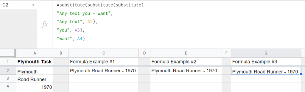
will work as well!
Merging cells in Google Sheets – FAQ
Let’s now go through some common questions you may be asking yourself.
How to remove merge cells in Google Sheets (unmerge cells)
Unmerging cells is similar to merging them in the first place. Do the following steps:
- Select the cells you want to unmerge (if you want to unmerge all cells in a sheet, click ctrl+A (Windows) or cmd+A (Mac) to select all cells. Don’t worry, nothing will happen to cells that weren’t merged in the first place.
- Pull up the Format menu or use the shortcut from the menu and choose Unmerge Cells.

Note: if any data was lost while merging data, you won’t get it back by simply unmerging a cell. You will need to click Undo the needed number of times or retrieve an earlier version of a worksheet from the Version history.
How to merge cells in Google Sheets horizontally
To merge cells horizontally, select cells in one or more rows. Then, pull up the merge cell menu either from the shortcuts above or the Format menu and select Merge horizontally.

Here’s the outcome:
If you don’t want to lose any of the data in these cells, you will want to use the relevant function or operator. We discussed them in detail in the Formula to merge cells in Google Sheets chapter.
How to merge cells vertically in Google Sheets
Merging cells vertically works just about the same as for horizontal merge. Select the cells, and this time, select Merge vertically:
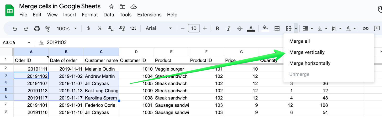
Here’s the outcome:

Same as above, if you want to preserve all underlying data, you’ll need to merge with relevant functions or an operator.
Why can’t I merge cells in Google Sheets?
If the range of cells you want to merge spans multiple cells and columns, you’ll want to make sure that each selected row has the same number of selected columns. In other words, the selected area must be rectangular or square-like (can’t have any irregular shape).
For example, you can’t highlight an area like below and merge it, even if it would make sense for your analysis. You’ll know it when you look at the Merge cells icon that will be grayed out.

This limitation can be overcome with the formulas we discussed above.
Likewise, you can’t merge cells if they’re not adjacent.

A simple CONCATENATE function, for example, would help overcome this problem.
What if I want to merge cells with date and time?
JOIN and TEXTJOIN functions are the best options to concatenate cells with date and time values. The SUBSTITUTE approach will also do the job. Check out the following formulas to merge two cells, A2 with date and A3 with time:
JOIN
=join(" ",A2:A3)TEXTJOIN=textjoin(" ",true,A2:A3)
SUBSTITUTE
substitute(substitute( "Date Time", "Date",A2), "Time",A3)
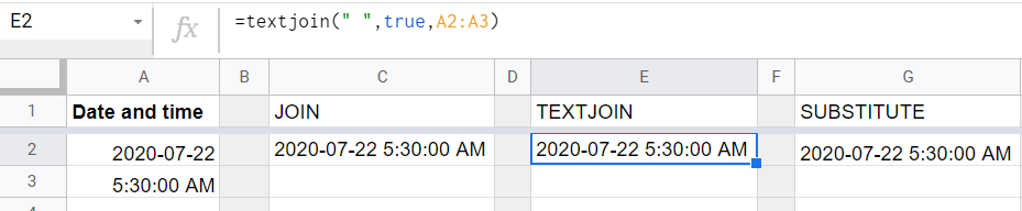
Other options – CONCAT, CONCATENATE and & – will return date-time values as simple numbers. For example, check out the CONCATENATE formula:
=concatenate(A2," ",A3)
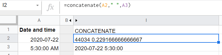
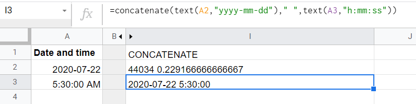
This can be fixed if you embed the TEXT function in your CONCATENATE formula as follows:
=concatenate(text(A2,"yyyy-mm-dd")," ",text(A3,"h:mm:ss"))
The same workaround works for CONCAT and & (ampersand) formulas.
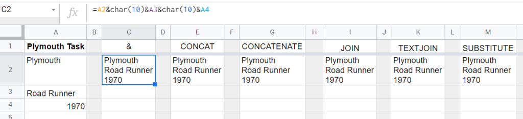
How to merge data strings with a line break: CHAR(10)
All the functions we mentioned concatenate data in line. However, there is an option to make a line break between the data you merge. For this, you’ll need to add CHAR(10) to your &/CONCAT/CONCATENATE/JOIN/TEXTJOIN formula. CHAR is a function to insert special characters.
Syntax
=char(table_number)
table_number– the special character number from the current Unicode table in decimal format.
Plymouth task
CHAR(10) inserts a line break. Let’s embed this into our merging formulas:
&
=A2&char(10)&A3&char(10)&A4
CONCAT:
=concat(A2, concat(char(10), concat(A3, concat(char(10),A4)))
CONCATENATE:
=concatenate(A2,char(10),A3,char(10),A4)
JOIN:
=join(char(10),A2,A3,A4)
TEXTJOIN:
=textjoin(char(10),true,A2,A3,A4)
SUBSTITUTE:
=substitute(substitute(substitute(substitute( "brand-model-year", "brand", A2), "model", A3), "year", A4), "-",char(10))
How to merge columns in Google Sheets
There’s no native functionality to merge columns in Google Sheets. None of the functions we discussed will also handle the job on its own. However, if you combine &, CONCAT, or SUBSTITUTE with ARRAYFORMULA, you’ll get the result. Let’s see how this works in practice.
But first, we’ll need to import some raw data to Google Sheets so that we can use it in our example. We’ll transfer data automatically with Coupler.io, a popular data analytics and integration platform. Coupler.io collects data via over 200+ integrations with apps like Airtable, Facebook Ads, GA4, HubSpot, and more. It allows you to transform and then load it into your spreadsheet. Other destinations include Excel, BigQuery, and Looker Studio.
Merge columns in Google Sheets – preparing data
We will export data from Airtable. See the complete list of the available integrations.
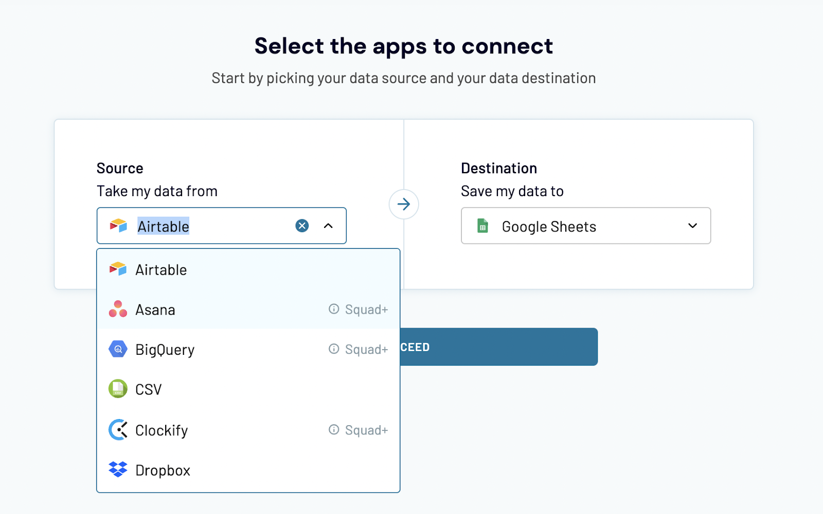
To export data, create a Coupler.io account for free.
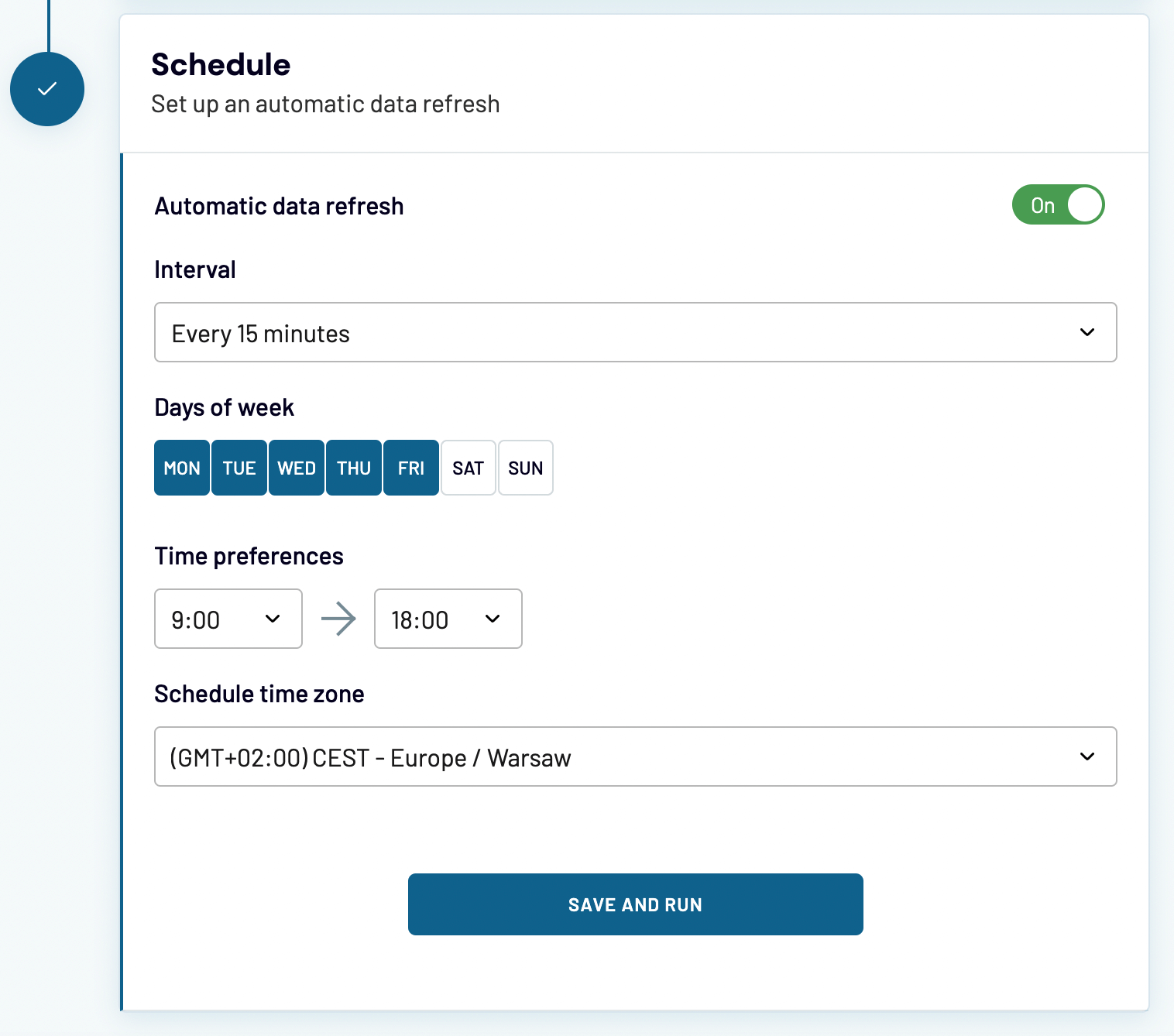
Then, connect to the app you want to fetch the data from. You can even move data between different Google Sheets files if you’d like. Apply the needed transformations – add or remove columns, apply filters, sort, and more.

You can also opt to refresh the data according to a schedule – for example, daily or hourly.
In the end, run the importer. Great! Now our data is transferred to Google Sheets, so we are ready to merge columns.
How to merge two columns in Google Sheets without losing data
We’ll now show you how to merge columns in Google Sheets. Since there are no native methods, there are several possible approaches. Here, we’re sharing arguably the easiest and most intuitive method. We basically merge two cells from separate columns and spread this behavior onto their entire columns.
Follow these steps to merge columns in Google Sheets:
- Type a formula to merge the first cells in each column (most likely, these will be cells from row 2 unless your dataset doesn’t have a header row). For example:
=C2&”_”&D2. Confirm that the cells merge correctly. - Wrap the formula in ARRAYFORMULA, editing the data ranges to cover the entire columns. In our case, it will be
=ARRAYFORMULA(C2:C&"_"&D2:D)
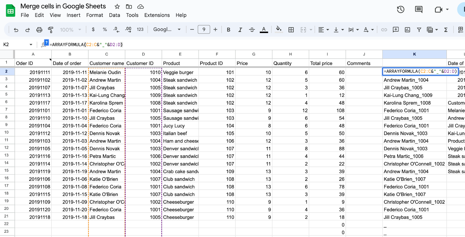
Hit Enter and the entire column will be populated with merged data. That’s it!
Merge columns in Google Sheets – more advanced scenario
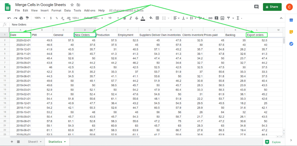
Now, let’s look at a more complex scenario. Again, we merge columns in Google Sheets, three of them to be specific. One of the fields is a date field which requires some special treatment depending on the method you choose.
We want to merge columns Date (A:A), New Orders (D:D), and Export Orders (L:L) using ” – ” as a delimiter.
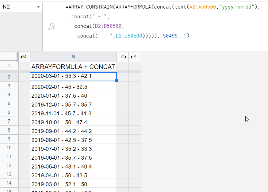
ARRAYFORMULA + CONCAT
CONCAT can merge two cells only, and this pattern remains for columns as well. So, to concatenate three or more columns, we’ll need to use the workaround. Besides, don’t forget that CONCAT returns date-time values as simple numbers, so we’ll need to add TEXT to the formula:
=arrayformula( concat(text(A2:A,"yyyy-mm-dd"), concat(" - ", concat(D2:D, concat(" - ",L2:L)))))
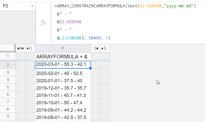
ARRAYFORMULA + &
For ampersand (&) we don’t need to invent any workarounds. However, the TEXT function for date-time is still needed:
=arrayformula( text(A2:A,"yyyy-mm-dd") &" - " &D2:D &" - " &L2:L)
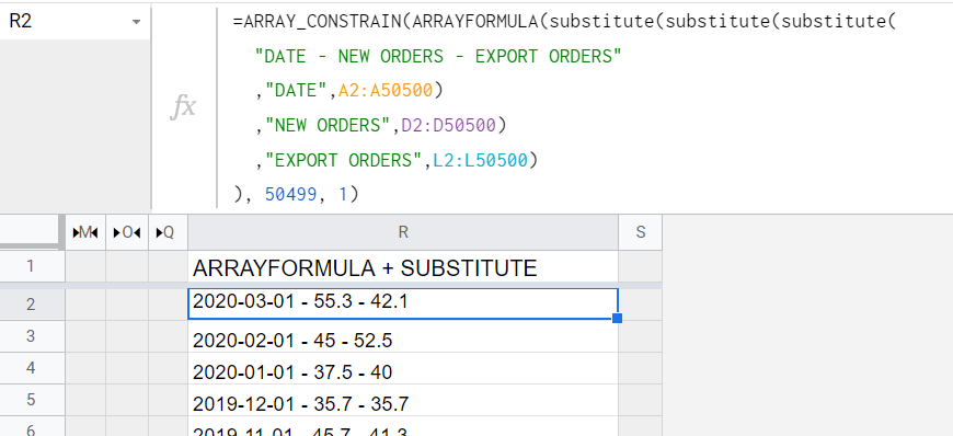
ARRAYFORMULA + SUBSTITUTE
Specify the merge_pattern and add ARRAYFORMULA:
=arrayformula(substitute(substitute(substitute( "DATE - NEW ORDERS - EXPORT ORDERS" ,"DATE",A2:A) ,"NEW ORDERS",D2:D) ,"EXPORT ORDERS",L2:L))
CONCATENATE, JOIN, or TEXTJOIN combined with ARRAYFORMULA don’t work. If you use either of these functions to merge columns, they will return all values from columns merged in a row.
Merge columns vertically with an array and semicolon
Vertical merge means that the data from several columns will be appended to each other in a single column. Use an array with a semicolon as a separator to merge column ranges.
Note: This method allows you to merge column ranges (not entire columns) vertically.
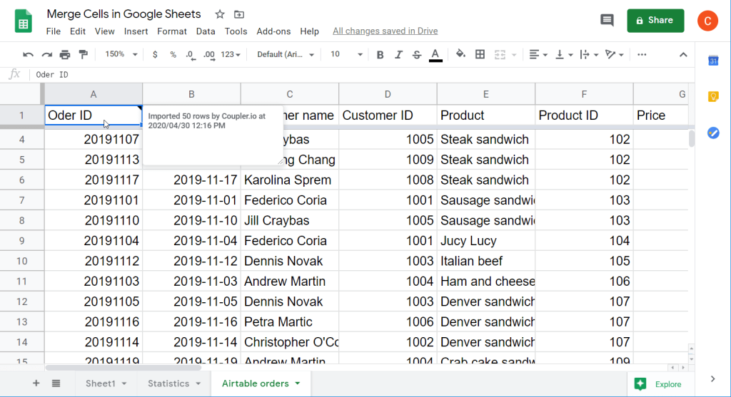
As an example, we’ll use a dataset imported from Airtable to Google Sheets.
Syntax
={column_range#1;column_range#2;column_range#3…}
Formula example
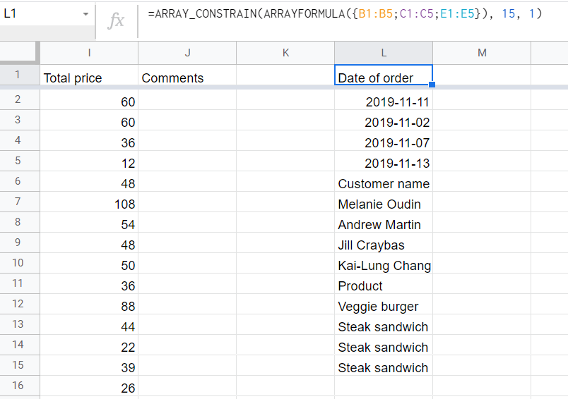
Let’s merge the following data ranges: B1:B5, C1:C5, E1:E5
={B1:B5;C1:C5;E1:E5}
Tip: If you’re merging column ranges with duplicate values, use the UNIQUE function to remove duplicates. Here is the formula syntax:
=unique({column_range#1;column_range#2;column_range#3…})
Thanks for reading!