VLOOKUP is a wonderful invention that saves you plenty of time and makes your calculations so much more efficient. At some point, however, you may come across its limitations too. These often appear when the values you search for are only approximate. In situations like that, Excel VLOOKUP wildcards are very handy.
Join us as we discuss the common use cases for using wildcards and explain each available type in detail.
What is Excel VLOOKUP wildcard?
Wildcards in Excel are a set of characters used to denote one or more other characters. They’re useful when you want to perform a VLOOKUP with just a partial match.
For example, you’re searching for certain data on your employee but only know their first name. Or – you want to scan a dataset and return the first result matching a certain pattern.
Let’s look at a more specific example. We have a dataset with thousands of employees in our firm. For some calculations, we need to include the salary of Ms. Ellie but aren’t exactly sure how her last name was spelled.
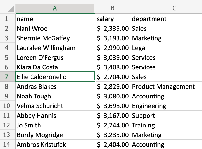
Misspelling it would result in an error. To avoid that, we will use a wildcard in a VLOOKUP formula:
=VLOOKUP("Ellie*",A:C,2,FALSE)
The function above searches for any record starting with “Ellie” and returns the salary for the first result found. Asterisk (*) stands for any number of characters.
To be more confident that we don’t accidentally capture data for another Ellie, it probably makes sense to make the search query more specific, e.g.
=VLOOKUP("Ellie Cal*",A:C,2,FALSE)
In another example, let’s say we want to return the department name for Ms. Klara Da Costa from the table above (row 6). Unfortunately, in our ignorance, we aren’t quite sure if her first name is spelled with ‘K’ or ‘C’. We can fix that by using another wildcard:
=VLOOKUP("?lara Da Costa",A:C,3,FALSE)
This search will capture the first Klara Da Costa or Clara Da Costa on the list but will ignore any employees with a longer first name, e.g., Phullara or Dulara. This is because a question mark (?) stands for a single character.
There’s one more Excel VLOOKUP wildcard available – ~ (tilde). We’ll explain the differences between all three with more examples in the following chapters.
Note: wildcards only work with text. For numerical values in VLOOKUP, it’s better to use logical expressions or VLOOKUP approximate matches.
Excel VLOOKUP wildcard with partial match vs approximate match
Now, you may be thinking – VLOOKUP itself has a setting that allows looking for only an approximate match. It’s the last argument of the function that accepts two inputs:
- TRUE (default) – search for an approximate match
- FALSE – search for an exact match
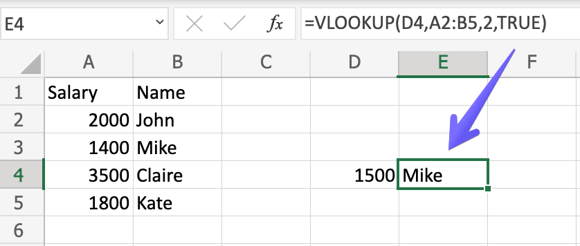
However, the said approximate match only works with numerical values. For example, in the following table, we search for an employee making $1,500. No one does, but VLOOKUP returns Mike, who earns the highest salary lower than the number we requested:
It won’t, however, work for text values. For example, if we were to search for the salary of an employee whose name starts with “Jo”, we would get a #N/A error.
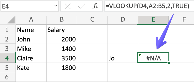
The right way to look for them would be with Excel VLOOKUP wildcards, searching for “Jo*” or “Jo??”.
Excel VLOOKUP wildcard examples
Okay, as promised, let’s go into more detail through different types of wildcards, examining some common examples.
Excel VLOOKUP wildcard examples
Okay, as promised, let’s go into more detail through different types of wildcards, examining some common examples. These examples are based on business data scenarios you might encounter in your day-to-day work.
Before we dive in, it’s worth noting that in real business environments, you’re often working with data from multiple sources like CRMs, accounting software, or e-commerce platforms. Rather than manually copying and pasting this data, use Coupler.io to import and consolidate information from over 60 cloud sources directly into Excel. This data and reporting solution lets you create automated data flows to apply these VLOOKUP wildcard techniques. Coupler.io saves time and ensures your analyses are always based on fresh information. Try it right away for free! Select the desired source app in the form below and follow the in-app instructions to load data to Excel.
Now, let’s explore how to leverage wildcards in VLOOKUP functions:
Excel VLOOKUP wildcard search with ‘*’ (asterisk)
Asterisk (*) is a very common wildcard in Excel. It represents any number of characters, including zero characters. For example, *east can point to the Southeast, Northeast, and East itself.
For a VLOOKUP example, let’s imagine that we’re running a clothing store. We have a long list of products with their SKU (stock keeping unit), sales volume, and prices, all sorted by the sales descending. We want to fetch the sales volume for the top-selling product in each category.
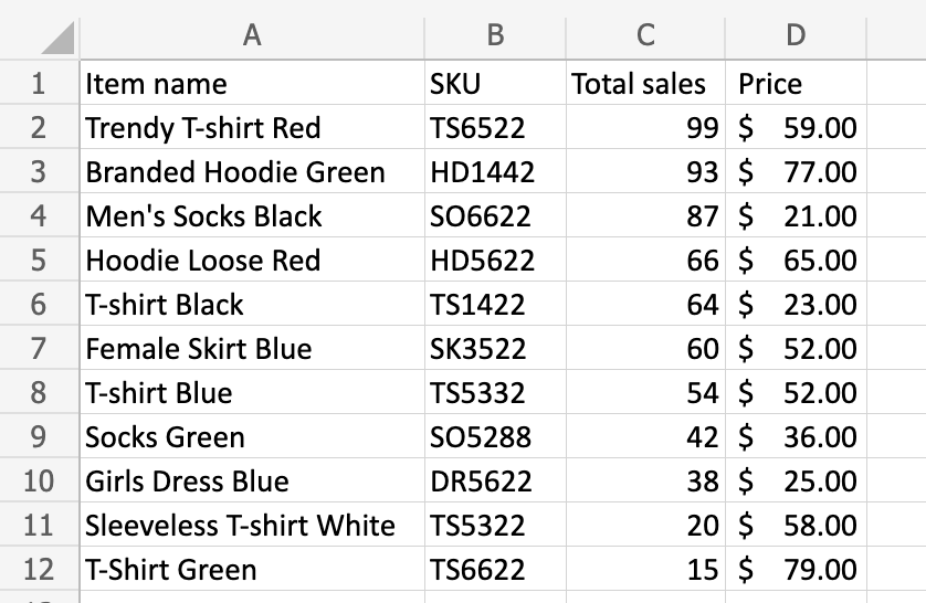
The first two letters of each product’s SKU indicate its category – for example, TS are t-shirts. Using it, we can write a VLOOKUP formula using an asterisk wildcard:
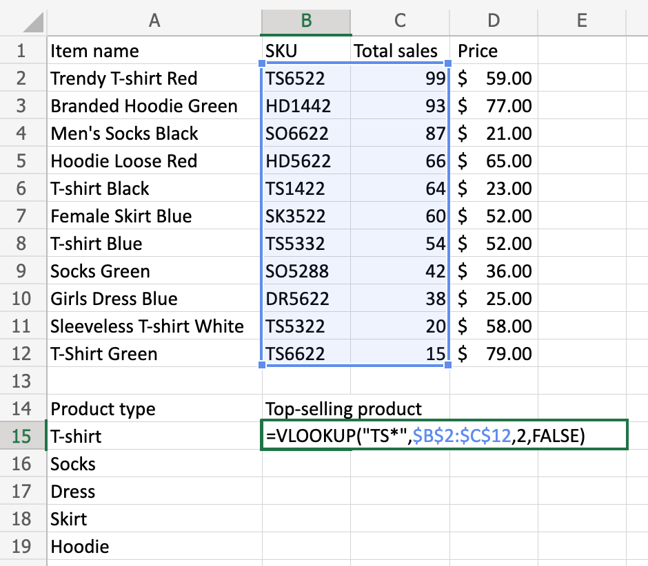
Then, we just stretch the formula onto the rest of the categories and update their first parameter.
Excel VLOOKUP with wildcard using ‘?’ (question mark)
A question mark wildcard denotes a single character. For example, searching for “Mi?e” would return “Mike”, “Mice”, “Mile”, “Mine”, or a few others. A question mark wildcard is useful when you know a bit more about what you’re searching for and, thus, can narrow down the results.
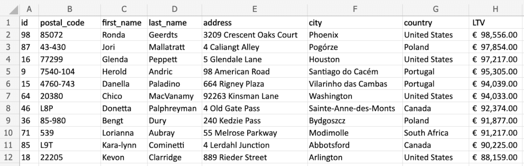
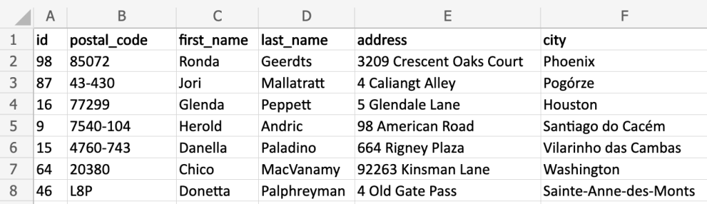
Let’s look at an example. Using Coupler.io, we’ve exported our list of customers from HubSpot, along with their LTV (lifetime value). This no-code tool lets you fetch data from Pipedrive, Salesforce, Airtable, QuickBooks, Jira, Shopify, and many other apps. Check the complete list of Microsoft Excel integrations and try it out for free.
Now, in a separate tab, we want to collect the LTV for the top customers from particular areas. For starters, we’re interested in checking the LTV for customers in the Portuguese town of Vilarinhos das Cambas and also its surrounding area. You can see the top performer in row 6 below.
Having done some research, we know that postal (zip) codes for that area always start with “4760-”. So we write the VLOOKUP formula as follows:
=VLOOKUP("4760-???",B:H,7,FALSE)
If we used an asterisk instead (e.g., “4760-*”), we could have accidentally captured other postal codes meeting the criteria – e.g., “4760-1” or “4760-57882AB”. Those could have been clients from some very different parts of the world,d which would skew our data.
How to use ~ (tilde) wildcard in Excel VLOOKUP formula?
There’s a third type of Excel VLOOKUP wildcards although much less frequently used than the other two. Tilde (~) is used to nullify the effects of the other wildcards. Why would you do that, though?
Let’s look at an earlier table exported from our CRM using Coupler.io. Due to some internal procedures, we started adding an asterisk to some country names. Let’s say this indicates that these customers are in our key markets and we want to be able to filter them out more easily.
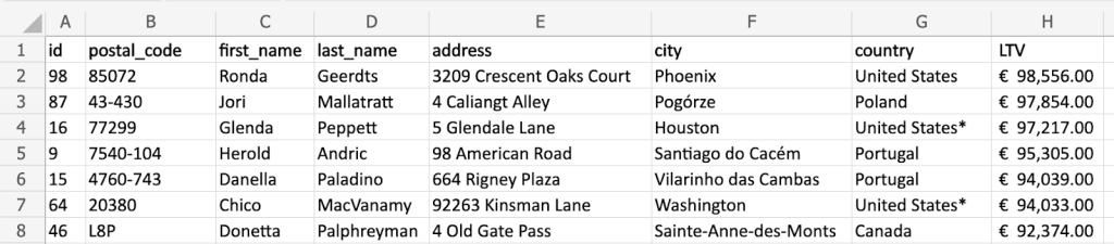
To find the top customer from such key markets in the United States, we could technically write the following function:
=VLOOKUP("United States?",G:H,2,FALSE)
It would correctly fetch the LTV for the third customer on the list. However, if we had another entry earlier on the list with, for example, “United States1” in the country field, VLOOKUP would pick it up first. For that reason, a tilde Excel VLOOKUP wildcard is used to nullify the effects of the other wildcards.
=VLOOKUP("United States~*",G:H,2,FALSE)
The function above would specifically search for “United States*” in column G, ignoring any other characters towards the end of the phrase.
Excel VLOOKUP Wildcard not working – troubleshooting
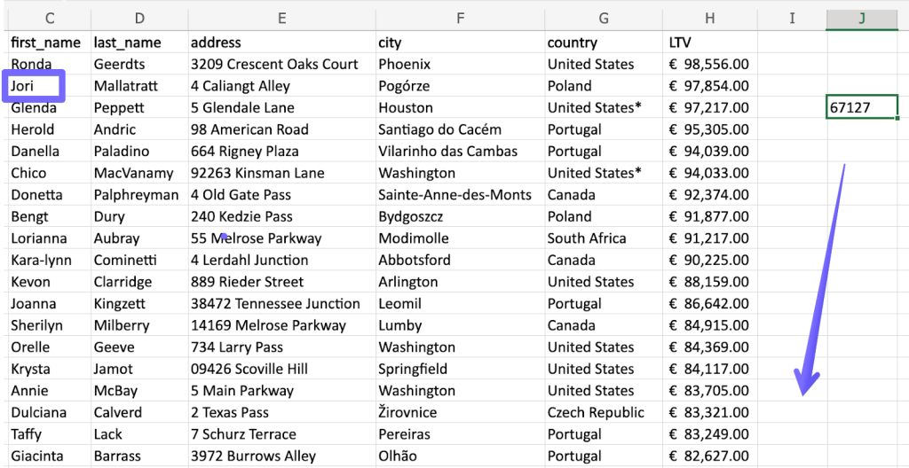
Probably the most common error when working with Excel VLOOKUP wildcards is choosing the approximate match (TRUE) setting in the general VLOOKUP syntax. For example:
=VLOOKUP(“Jo*”,C:H,6,TRUE)
Running this on our earlier dataset, we didn’t stop at Jori from the third row but (accidentally) picked up an LTV value for a contact way down the list.
As a reminder, approximate match only works with numerical values. When you set TRUE as a parameter, Excel translates the input into a number and tries to match it with a value in the chosen range. It’s easy to miss it because VLOOKUP will likely return some value rather than an error – it’s just that it’s not going to be the value you were looking for.
Another common issue with VLOOKUP itself is when the column to search through is to the right of the desired output. For example, we can’t use VLOOKUP to search for a specific first_name and expect the function to return an ID.
If possible, we need to reposition the fields so that the output column is to the right from the searched values. In a rare scenario, the output can also be in the same column but never to the left. If you can’t reposition the columns in a dataset, you can use INDEX and MATCH functions instead to reference the right fields.
Sometimes, VLOOKUP issues stem from inconsistent or poorly structured source data. If you’re frequently experiencing problems with data pulled from business systems, consider using Coupler.io to import and transform your data before applying VLOOKUP formulas. Coupler.io can help normalize your data during the import process, making it more consistent and reliable for VLOOKUP operations.

Automate data flows to Excel with Coupler.io
Get started for freeExcel VLOOKUP wildcard – wrapping up
To wrap up, let’s recap the three wildcards you can use with Excel VLOOKUP:
- Asterisk (*) represents 0 or any number of characters
- Question mark (?) represents a single character
- Tilde (~) nullifies the previous two wildcards, allowing you to treat them as regular text inputs.
On another note – if you spend your precious time importing data manually into Excel, there’s probably a more efficient way to do this. Coupler.io lets you set up automated data imports that pull data from your apps on the schedule you choose. It takes just a few minutes to set up and the importers will run forever, with zero effort on your side. You can focus on your latest data while we take care of the rest.