Compare Two Columns in Excel Using VLOOKUP in 2023

Let’s say you have two columns with some textual or numeric values and you need to identify which values are present in both columns and which aren’t. The VLOOKUP function will help you complete this task.

How to VLOOKUP two columns in Excel

We imported a dataset from Google Sheets to Excel using Coupler.io, a solution for automatic data exports from multiple apps and sources.

Read more about Microsoft Excel integrations for data export on a schedule.

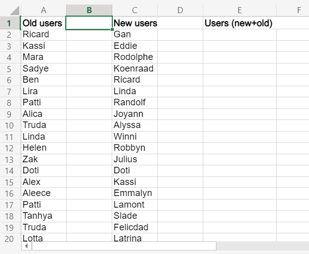
On the dataset, we have two columns: Old users and New users. What we need is to compare the values from these columns to identify duplicates – values that are present in both columns.

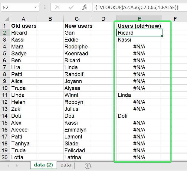
We can do this using the VLOOKUP function applied as an array formula. Select an array, which will be not less than the arrays in your VLOOKUP formula, insert the following formula to the formula bar and press Ctrl+Shift+Enter for Windows (Command+Return for Mac) – this will apply an array formula in Excel:

=VLOOKUP(A2:A66,C2:C66,1,FALSE)

• A2:A66– a lookup array
• C2:C66 – the range to look up
• 1 – the column to return the matching values from

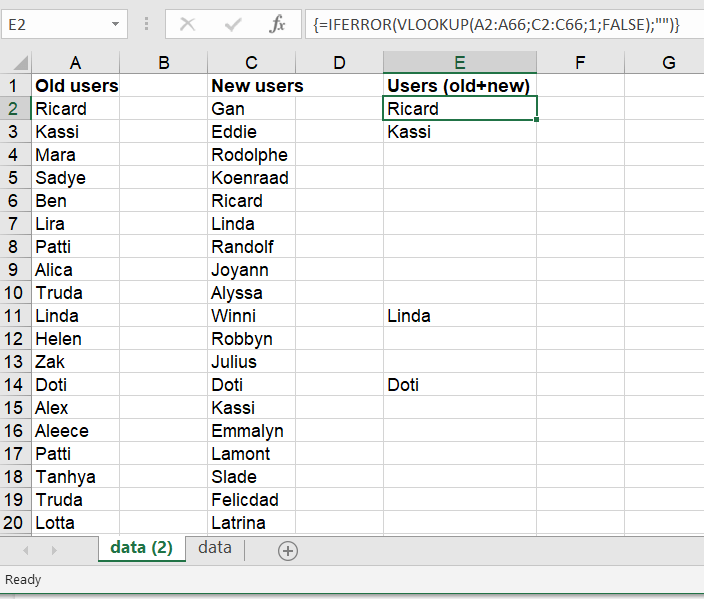
To get rid of #N/A, let’s nest our VLOOKUP formula with IFERROR as follows:

=IFERROR(VLOOKUP(A2:A66,C2:C66,1,FALSE),"")

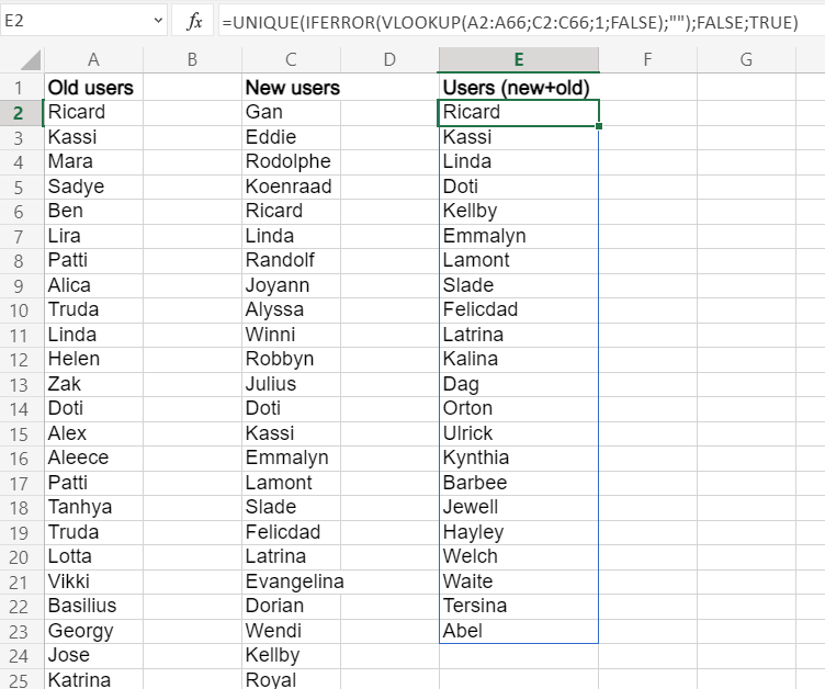
It would also be great to exclude empty cells in the array. You can do this using the UNIQUE function, which is available in Excel 365 or Excel Online. Here is how the formula will look:

=UNIQUE(IFERROR(VLOOKUP(A2:A66,C2:C66,1,FALSE);""),FALSE,TRUE)