Ranges are a key concept in Excel, and knowing how to work with them is essential for anyone who wants to program or automate their work using Excel VBA.
In this tutorial, we’ll take a look at how to work with Excel ranges in VBA. We’ll start by discussing what a Range object is. Then, we’ll look at the different ways of referencing a range. Lastly, we’ll explore various examples of how to work with ranges using VBA code.
Excel VBA: The Range object
The Excel VBA Range object is used to represent a range in a worksheet. A range can be a cell, a group of cells, or even all the 17,179,869,184 cells in a sheet.
When programming with Excel VBA, the Range object is going to be your best friend. That’s because much of your work will focus on manipulating data within sheets. Understanding how to work with the Range object will make it easier for you to perform various actions on cells, such as changing their values, sorting, or doing a copy-paste.
The following is the Excel object hierarchy:
| Application > Workbook > Worksheet > Range |
You can see that the Excel VBA Range object is a property of the Worksheet object. This means that you can access a range by specifying the name of the sheet and the cell address you want to work with. When you don’t specify a sheet name, by default Excel will look for the range in the active sheet. For example, if Sheet1 is active, then both of these lines will refer to the same cell range:
Range("A1")
Worksheets("Sheet1").Range("A1")
Let’s have a closer look at how to reference a range in the section below.
Referencing a range of cells in Excel VBA
Referring to a Range object in Excel VBA can be done in several ways. We’ll discuss the basic syntax and some alternatives that you might want to use, depending on your needs.
Excel VBA: Syntax for specifying a cell range
To refer to a range that consists of one cell, for example, cell D5, you can use the syntax below:
Range("D5")
To refer to a range of cells, you have two acceptable syntaxes. For example, A1 through D5 can be specified using any one below:
Range("A1:D5")
Range("A1", "D5")
To refer to a range outside the active sheet, you need to include the worksheet name. Here’s an example:
Worksheets("Sheet1").Range("A1:D5")
To refer to an entire row, for example, Row 5:
Range("5:5")
To refer to an entire column, for example, Column D:
Range("D:D")
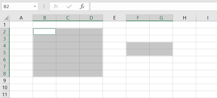
Excel VBA also allows you to refer to multiple ranges at once by using a comma to separate each area. For example, see the below syntax used for referring to all ranges shown in the image:
Range("B2:D8, F4:G5")
Tip: Notice that all of the syntaxes above use double quotes to enclose the range address. To make it quicker for you to type, you can use shortcuts that involve using square brackets without quotes, as shown in the table below:
| Syntax | Shortcut |
|---|---|
Range("D5") | [D5] |
Range("A1:D5") | [A1:D5] |
Range("5:5") | [5:5] |
Range("B2:D8, F4:G5") | [B2:D8, F4:G5] |
Excel VBA: Referencing a named range
You have probably already used named ranges in your worksheets. They can be found under Name Manager in the Formulas tab.
To refer to a range named MyRange, use the following code:
Range("MyRange")
Remember to enclose the range’s name in double quotes. Otherwise, Excel thinks that you’re referring to a variable.
Alternatively, you can also use the shortcut syntax discussed previously. In this case, double quotes aren’t used:
[MyRange]
Excel VBA: Referencing a range using the Cells property
Another way to refer to a range is by using the Cells property. This property takes two arguments:
Cells(Row, Column)
You must use a numeric value for Row, but you may use either a numeric or string value for Column. Both of these lines refer to cell D5:
Cells(5, "D")
Cells(5, 4)
The advantage of using the Cells property to refer to ranges becomes clear when you need to loop through rows or columns. You can create a more readable piece of code by using variables as the Cells arguments in a looping.
Excel VBA: Referencing a range using the Offset property
The Offset property provides another handy means for referring to ranges. It allows you to refer to a cell based on the location of another cell, such as the active cell.
Like the Cells property, the Offset property has two parameters. The first determines how many rows to offset, while the second represents the number of columns to offset. Here is the syntax:
Range.Offset(RowOffset, ColumnOffset)
For example, the following code refers to cell D5 from cell A1:
Range("A1").Offset(4,3)
The negative numbers refer to cells that are above or below the range of values. For example, a -2 row offset refers to two rows above the range, and a -1 column offset refers to a column to the left of the range. The following example refers to cell A1:
Range("D3").Offset(-2, -3)
If you need to go over only a row or a column, but not both, you don’t have to enter both the row and the column parameters. You can also use 0 as one or both of the arguments. For example, the following lines refer to D5:
Range("D5").Offset(0, 0)
Range("D2").Offset(3, 0)
Range("G5").Offset(, -3)
Excel VBA Range: How to & examples
Let’s take a look at some of the most common range examples. These examples will show you how to use VBA to select and manipulate ranges in your worksheets. Some of these examples are complete procedures, while others are code snippets that you can just copy-paste to your own Sub to try.
Excel VBA: Select a range of cells
To select a range of cells, use the Select method.
The following line selects a range from A1 to D5 in the active worksheet:
Range("A1:D5").Select
To select a range from A1 to the active cell, use the following line:
Range("A1", ActiveCell).Select
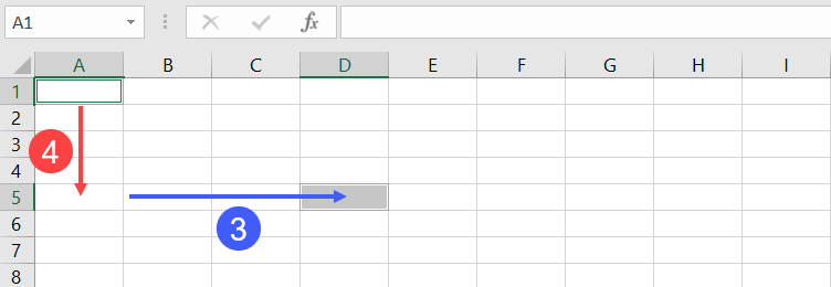
The following code selects from the active cell to 3 rows below the active cell and five columns to the right:
Range(ActiveCell, ActiveCell.Offset(3, 5)).Select
It’s important to note that when you need to select a range on a specific worksheet, you need to ensure that the correct worksheet is active. Otherwise, an error will occur. For example, you want to select B2 to J5 on Sheet1. The following code will generate an error if Sheet1 is not active:
Worksheets("Sheet1").Range("B2:J5").Select
Instead, use these two lines of code to make your code work as expected:
Worksheets("Sheet1").Activate
Range("B2:J5").Select
Excel VBA: Set values to a range
The following statement sets a value of 100 into cell C7 of the active worksheet:
Range("C7").Value = 100
The Value property allows you to represent the value of any cell in a worksheet. It’s a read/write property, so you can use it for both reading and changing values.
You can also set values of a range of any size. The following statement enters the text “Hello” into each cell in the range A1:C7 in Sheet2:
Worksheets("Sheet2").Range("A1:C7").Value = "Hello"
Value is the default property for a Range object. This means that if you don’t provide any properties in your range, Excel will use this Value property.
Both of the following lines enter a value of 100 into cell C7 of the active worksheet:
Range("C7").Value = 100
Range("C7") = 100
Excel VBA: Copy range to another sheet
To copy and paste a range in Excel VBA, you use the Copy and Paste methods. The Copy method copies a range, and the Paste method pastes it into a worksheet. It might look a bit complicated but let’s see what each does with an example below.
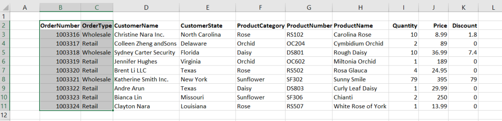
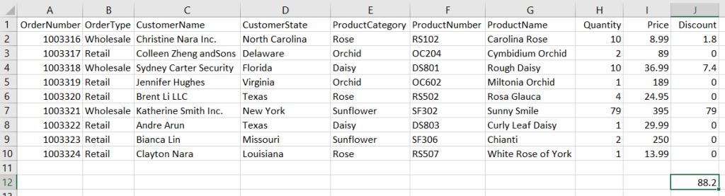
Let’s say you have Orders data, as shown in the below screenshot, which is imported from Airtable every day using Coupler.io. This tool allows users to do it automatically on the schedule they want with just a few clicks and no coding required.

Streamline your data automation with Coupler.io
Get started for freeIn addition, they can combine data from other different sources (such as Jira, Mailchimp, etc.) into one destination for analysis purposes.
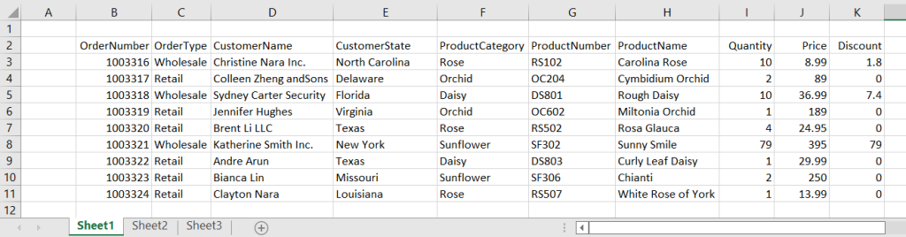
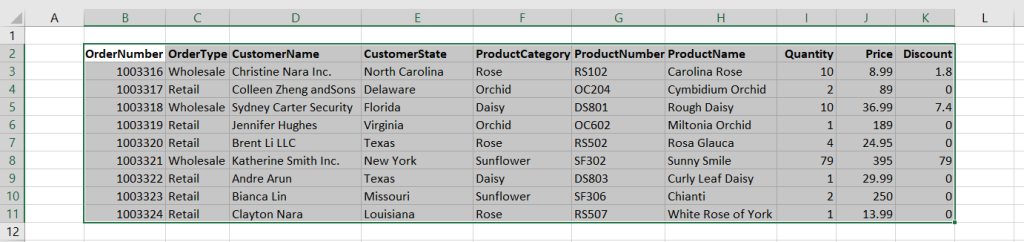
As you can see, the data starts from B2. You want to copy only range B2:C11 and paste them to Sheet2 at the same address. The following is an example Sub you can use:
Sub CopyRangeToAnotherSheet()
    Sheets("Sheet1").Activate
    Range("B2:C11").Select
    Selection.Copy

    Sheets("Sheet2").Activate
    Range("B2").Select
    ActiveSheet.Paste
End Sub
Alternatively, you can also use a single line of code as shown below:
Sub CopyRangeToAnotherSheet2()
    Worksheets("Sheet1").Range("B2:C11").Copy Worksheets("Sheet2").Range("B2")
End Sub
The above Sub procedure takes advantage of the fact that the Copy method can use an argument that corresponds to the destination range for the copy operation. Notice that actually, you don’t have to select a range before doing something with it.
Excel VBA: Dynamic range example
In many cases, you may need to copy a range of cells but don’t know exactly how many rows and columns it has. For example, if you use Coupler.io or other integration tools to import data from an external app into Excel on a daily schedule, the number of rows may change over time.
How can you determine this dynamic range? One solution is to use the CurrentRegion property. This property returns an Excel VBA Range object within its boundaries. As long as the data is surrounded by one empty row and one empty column, you can select it with CurrentRegion.
The following line selects the contiguous range around Cell B2:
Range("B2").CurrentRegion.Select
Now, let’s say you want to select only Columns B and C of the range, and from the second row, you can use the following line:
Range("B2", Range("C2").End(xlDown)).Select
You can now do whatever you want with your selected range — copy or move it to another sheet, format it, and so on.
If you want to find the last row of a used range using Excel VBA, it’s also possible without selecting anything. Here’s the line you can use to find the row number of Column B’s last row data:
' Find the row number of Column B's last row data
RowNumOfLastRow = Cells(Rows.Count, 2).End(xlUp).Row


' Result: 11
MsgBox RowNumOfLastRow
Excel VBA: Loop for each cell in a range
For looping each cell in a range, the For Each loop is an excellent choice. This type of loop is great for looping through a collection of objects such as cells in a range, worksheets in a workbook, or other collections.
The following procedure shows how to loop through each cell in Range B2:K11. We use an object variable named Obj, which refers to the cell being processed. Within the loop, the code checks if the cell contains a formula and then sets its color to blue.
Sub LoopForEachCell()
    Dim obj As Range
    For Each obj In Range("B2:K11")
        If obj.HasFormula Then obj.Font.Color = vbBlue
    Next obj
End Sub
Excel VBA: Loop for each row in a range
When looping through rows (or columns), you can use the Cells property to refer to a range of cells. This makes your code more readable compared to when you’re using the Range syntax.
For example, to loop for each row in range B2:K11 and bold all the cells from Column I to K, you might write a loop like this:
Sub LoopForEachRow()
    For i = 1 To 11
        Range("I" & i & ":K" & i).Font.Bold = True
    Next i
End Sub
Instead of typing in a range address, you can use the Cells property to make the loop easier to read and write. For example, the code below uses the Cells and Resize properties to find the required cell based on the active cell:
Sub LoopForEachRow2()
    For i = 1 To 11
        Cells(i, "I").Resize(, 3).Font.Bold = True
    Next i
End Sub
Excel VBA: Clear a range
There are three ways to clear a range in Excel VBA.
The first is to use the Clear method, which will clear the entire range, including cell contents and formatting.
The second is to use the ClearContents method, which will clear the contents of the range but leave the formatting intact.
The third is to use the ClearFormats method, which will clear the formatting of the range but leave the contents intact.
For example, to clear a range B1 to M15, you can use one of the following lines of code below, based on your needs:
Range("B1:M15").Clear
Range("B1:M15").ClearContents
Range("B1:M15").ClearFormats
Excel VBA: Delete a range
When deleting a range, it differs from just clearing a range. That’s because Excel shifts the remaining cells around to fill up your deleted range.
The code below deletes Row 5 using the Delete method:
Range("5:5").Delete
To delete a range that is not a complete row or column, you have to provide an argument (such as xlToLeft, xlUp — based on your needs) that indicates how Excel should shift the remaining cells.
For example, the following code deletes cell B2 to M10, then fills the resulting gap by shifting the other cells to the left:
Range("B2:M10").Delete xlToLeft
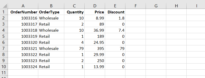
Excel VBA: Delete rows with a specific condition in a range
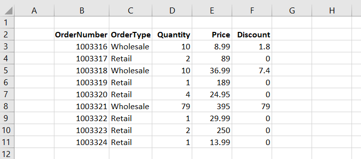
You can also use a VBA code to delete rows with a specific condition. For example, let’s try to delete all the rows with a discount of 0 from the below sheet:
Here’s an example Sub you may want to use:
Sub DeleteWithCondition()
    For i = 3 To 11
        If Cells(i, "F").Value = 0 Then
            Cells(i, 1).EntireRow.Delete
        End If
    Next i
End Sub
The above code loops from Row 3 to 11. In each loop, it checks the discount value in Column F and removes the entire row if the value equals 0.
Excel VBA: Find values in a range
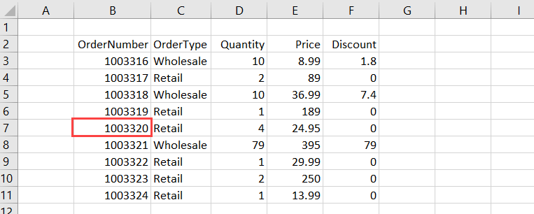
With the below data, suppose you want to find if there is an order with OrderNumber equal to 1003320 and output its cell address.
You can use the Find method in this case, as shown in the below code:
Sub FindOrder()
    Dim Rng As Range

    Set Rng = Range("B3:B11").Find("1003320")

    If Rng Is Nothing Then
        MsgBox "The OrderNumber not found."
    Else
        MsgBox Rng.Address
    End If

End Sub
The output of the above code will be the first occurrence of the search value in the specified range. If the value is not found, a message box showing info that the order is not found will appear.
Excel VBA: Add al?h?b?t? using R?ng? .Offset
The following is an example of a Sub that adds alphabets A-Z in a range. The code uses Offset to refer to a cell below the active cell in a loop.
Sub AddAlphabetsAZ()
    Dim i As Integer

    ' Use 97 To 122 for lowercase letters
    For i = 65 To 90
        ActiveCell.Value = Chr(i)
        ActiveCell.Offset(1, 0).Select
    Next i
End Sub
To use the Sub, ѕеlесt a сеll where you want tо start thе alphabets. Then, run it by pressing F5. The code will insert A-Z to the cells downward.
Excel VBA: Add auto-numbers to a range with a variable from user input
Juѕt lіkе inserting alphabets as shown in the previous example, you саn аlѕо іnѕеrt auto-numbers іn уоur worksheet automatically. This can be helpful when you work with large data.
The following is an example of a Sub that adds auto-numbers to your Excel sheet:
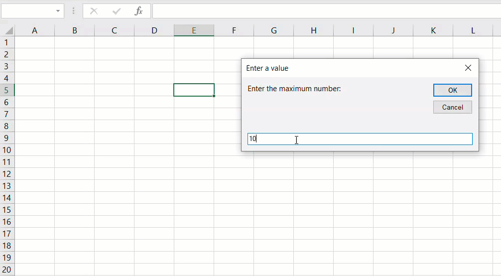
Sub AddAutoNumbers()
    Dim i As Integer

    On Error GoTo ErrorHandler

    i = InputBox("Enter the maximum number: ", "Enter a value")

    For i = 1 To i
        ActiveCell.Value = i
        ActiveCell.Offset(1, 0).Select
    Next i

ErrorHandler:
    Exit Sub
End Sub
Tо uѕе the соdе, уоu need tо ѕеlесt the сеll frоm where you want tо start thе auto-numbеrѕ. Then, run the Sub. In the message box that appears, enter the maximum value for the auto-numbers and сlісk OK.
Excel VBA: Sum a range
Imagine that you have written a Sub procedure to import Orders.csv into an Excel sheet:
Automate import of CSV to Excel without any coding with Coupler.io
Load data from 400+ sources to Excel with Coupler.io
Get started for freeYou want to sum up all the discount values and put the result in J12. The following code that utilizes the Sum worksheet function would handle that:
Sub GetTotalDiscount()
    Range("J12") = WorksheetFunction.Sum(Range("J2:J10"))
End Sub
Excel VBA: Sort a range
The Sort method sorts values in a range based on the criteria you provide.
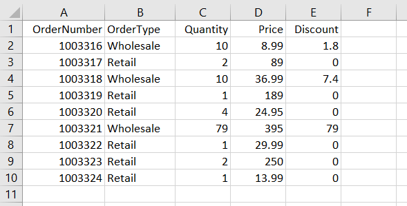
Suppose you have the following sheet:
To sort the above data based оn thе vаluеѕ іn Column D, you can use the following code:
Sub SortBySingleColumn()
    Range("A1:E10").Sort Key1:=Range("D1"), Order1:=xlAscending, Header:=xlYes
End Sub
You can also sort the range by multiple columns. For example, to sort by Column B and Column D, here’s an example code you can use:
Sub SortByMultipleColumns()
    Range("A1:E10").Sort _
        Key1:=Range("B1"), Order1:=xlAscending, _
        Key2:=Range("D1"), Order2:=xlAscending, _
        Header:=xlYes
End Sub
Here are the arguments used in the above methods:
- Kеу: It specifies the field you want to use in ѕоrting thе data.
- Ordеr: It ѕресіfies whеthеr уоu wаnt tо sort the dаtа іn аѕсеndіng or dеѕсеndіng order.
- Header: It spесіfies whеthеr уоur data hаѕ hеаdеrѕ оr nоt.
Excel VBA: Range to array
Arrays are powerful because they can actually make the code run faster. Especially when working with large data, you can use arrays to make all the processing happen in memory and then write the data to the sheet once.
For example, suppose you have the following sheet:
The following Sub uses a variable X, which is a Variant data type, to store the value of Range A2:E10. Variants can hold any type of data, including arrays.
Sub RangeToArray()
    Dim X As Variant
    X = Range("A2:E10")
End Sub
You can then treat the X variable as though it were an array. The following line returns the value of cell A6:
MsgBox X(5, 1)
' Result: 1003320
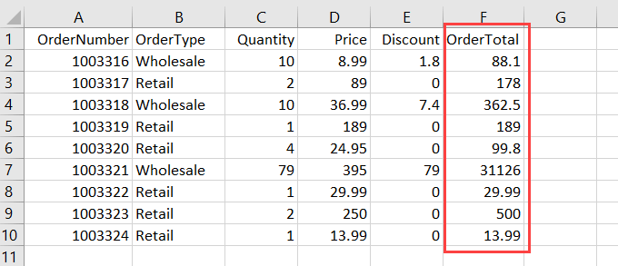
Now, let’s say you want to calculate the total order using the following calculation:
Quantity * Price - Discount
Rather than doing calculation and writing the result for each row using a looping, you can store the calculation result in an array OrderTotal as shown in the below code and write the result once:
Sub CalculateTotalOrder()
    Dim X As Variant, OrderTotal As Variant
    X = Range("A2:E10")

    ReDim OrderTotal(UBound(X))

    For i = LBound(X) To UBound(X)
        OrderTotal(i - 1) = X(i, 3) * X(i, 4) - X(i, 5)
    Next i

    Range("F1") = "OrderTotal"

    Range("F2").Resize(UBound(OrderTotal)) = _
        Application.Transpose(OrderTotal)

End Sub
Here’s the final result:
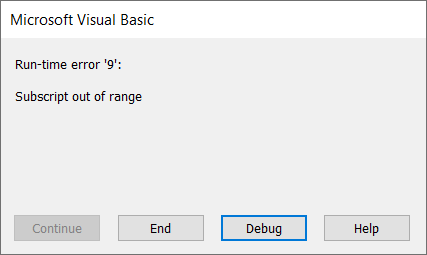
Subscript out of range: Excel VBA Runtime error 9
This error message often happens when you try to access a range of cells in a worksheet that has been deleted or renamed.
Let’s say your code expected a worksheet named Setting. For some reason, this sheet is renamed Settings. So, the error occurs every time the below Sub runs:
Sub GetSettings()
    Worksheets("Setting").Select
    x = Range("A1").Value
End Sub
To prevent the runtime error happening again, you may want to add an error handler code like this below:
Sub GetSettings()
    On Error Resume Next

    ws = Worksheets("Setting")
    Name = ws.Name

    If Not Err.Number = 0 Then
        MsgBox "Expected to find a Setting worksheet, but it is missing."
        Exit Sub
    End If
    On Error GoTo 0

    ws.Select
    x = Range("A1").Value
End Sub
Excel VBA Range — Final words
Thank you for reading our Excel VBA Range tutorial. We hope that you’ve found it helpful! And if there’s anything else about Excel programming or other topics that interest you, be sure to check out our other Excel tutorials.
In addition, you may find that Coupler.io is a valuable tool for you if you’re looking for an easy way to pull and combine your data from multiple sources into one destination for analysis and reporting. This tool also lets you specify the range address of your imported data so you can keep all of your calculations (including. formulas) in the sheets.
Thanks again for reading, and happy coding!
