Excel Vlookup Multiple Columns: Explanation + Examples

The Excel VLOOKUP function allows you to look up on one column at a time. And what if you need to return the matching values from two or more columns? This can be done quite easily. 

Excel vlookup on multiple columns – the logic of the lookup

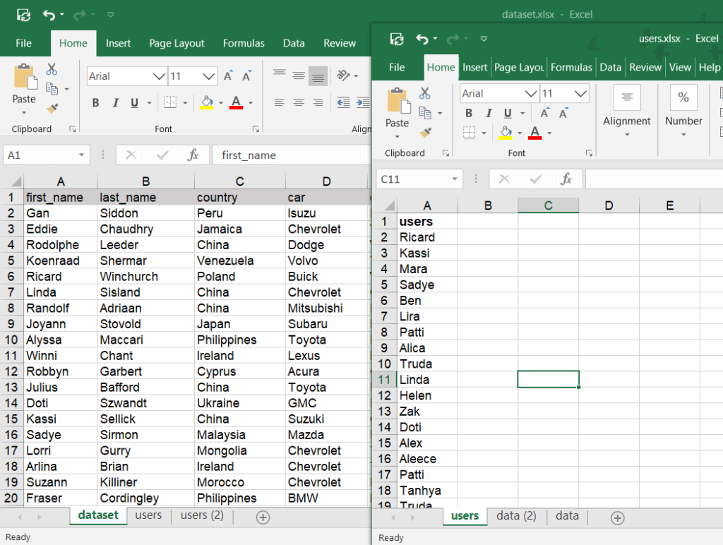
We have a dataset imported from BigQuery to Excel using Coupler.io, a solution for automatic data exports from multiple apps and sources.

Learn more about Coupler.io and check out other Microsoft Excel integrations available for data export on a schedule.

Our goal is to learn the car, color, and country for a specific user name. For this, we need to look up these three columns.

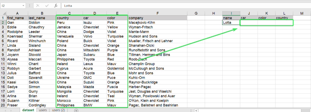
The basic format of the VLOOKUP only returns a single value. But a small tweak will do the job for us.

Excel VLOOKUP multiple columns syntax

=VLOOKUP("lookup_value",lookup_range, {col1,col2,col3…},[match])

• "lookup_value" – the value you want to look up vertically. Quotes are not used if you reference a cell as a lookup value.
• lookup_range – the data range where to search the "lookup_value" and the matching value. 
• {col1,col2,col3…} the numbers of the columns that contain the matching values to return. For example, if your range is D7:G18, D is the first column, E is the second one, and so on. You can change the order of columns to the one you need – for example, {5,3,6,2}
• To return the closest match, specify TRUE; to return the exact match, specify FALSE. The closest match (TRUE) is set by default.

How to vlookup multiple columns in Excel – example

Here is the VLOOKUP formula we have:

=VLOOKUP(I2,A:F,{4,5,3},FALSE)

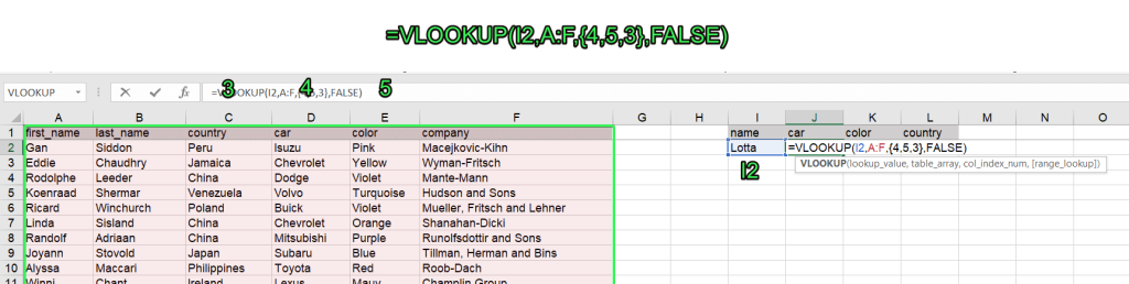
But you can’t just insert this formula into J2 cell and hit enter. This would only return one value. What you need to do is select a vertical array that corresponds to the number of columns in your VLOOKUP formula. In our case, we need to select three cells. After that, you can insert the formula to the formula bar and press Ctrl+Shift+Enter for Windows (Command+Return for Mac) – this will apply an array formula in Excel.

Excel Online vlookup to return multiple columns 

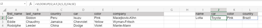
In Excel Online, VLOOKUP works almost the same way, but you don’t have to select an array and press the combination of buttons to implement it.

You can just insert the formula in one cell and press Enter => the matching values for the columns specified in the formula will be populated automatically.

Excel vlookup array on multiple columns in different workbooks

If your lookup values and lookup range are stored in different workbooks, the VLOOKUP function works the same way. The only difference is that you need to select the lookup range in the other spreadsheet.

For example, we have two workbooks

• “dataset” – contains the lookup range
• “users” – contains the array of lookup values

To vlookup the range in a separate workbook, complete the following steps:

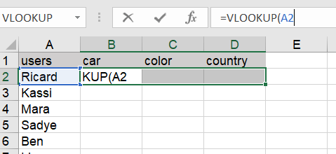
• Select the array B2:D2 in the “users” workbook. In the formula bar, type =vlookup( and specify the lookup value:

=VLOOKUP(A2

• Enter a comma/semicolon (depending on the list separator defined under your regional settings), click on the spreadsheet with the range you want to look up and select the desired range. In our case, the unfinished formula looks like this:

=vlookup(A2,[dataset.xlsx]dataset!$A:$F

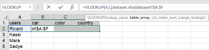
So, basically, you can manually type the range to lookup using the following sample:

[dataset.xlsx]dataset!$A:$F

• [dataset.xlsx] – name of the spreadsheet
• dataset! – name of the worksheet
• $A:$F – locked range to lookup

• To finalize the VLOOKUP formula, we need to enter the numbers of the columns to look up, and enter FALSE to return the exact match. Close the bracket and press Ctrl+Shift+Enter for Windows (Command+Return for Mac)

=vlookup(A2,[dataset.xlsx]dataset!$A:$F,{4,5,3},FALSE)

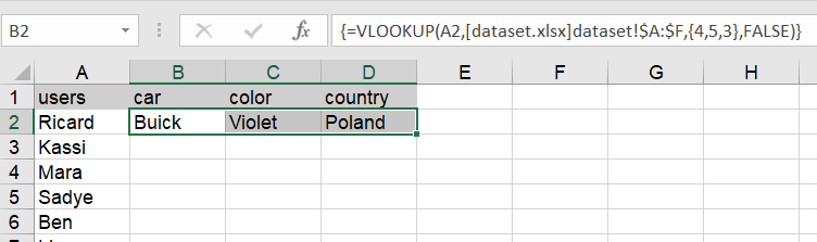
Now you can drag the formula down to return matching values for all the users.

Excel vlookup compare multiple columns

We already blogged about how to compare two columns in Excel using VLOOKUP. Let’s see how we can make a comparison of three columns. 

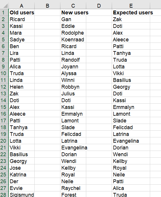
In the dataset, we have three columns: Old users, New users, and Expected users. VLOOKUP will help us compare the values from these columns to identify the values that are present in all of the columns.

The logic of the formula is the following:

• First we need to compare two columns and identify the matches
• Then, we need to compare the third column with the identified matches 

The same logic will apply for bigger numbers of columns to compare – you need to narrow down the comparison to two columns. In our case, the VLOOKUP formula will look as follows

=IFERROR(VLOOKUP(IFERROR(VLOOKUP(A:A,C:C,1,FALSE),""),E:E,1,FALSE),"")

• VLOOKUP(A:A,C:C,1,FALSE) – the comparison of columns A (first column) and B (second column). 
• E:E – the range to look up (third column) against the matching values returned from the comparison of the first and second columns 
• 1 – the column to return the matching values from
• IFERROR is used to replace the #N/A with blank cells

To implement the formula, select an array, which will be not less than the arrays in your VLOOKUP formula, insert the following formula to the formula bar and press Ctrl+Shift+Enter for Windows (Command+Return for Mac):

It would also be great to exclude empty cells in the array. You can do this using the UNIQUE function, which is available in Excel 365 or Excel Online. The other way is to apply this advanced array formula:

=IF(ISERROR(SMALL(IF(H2:H66<>"",ROW(H2:H66)-1),ROW(H2:H66)-1)),"",
INDEX(H2:H66,MATCH(SMALL(IF(H2:H66<>"",ROW(H2:H66)-1),ROW(H2:H66)-1),
IF(H2:H66<>"",ROW(H2:H66)-1),0)))

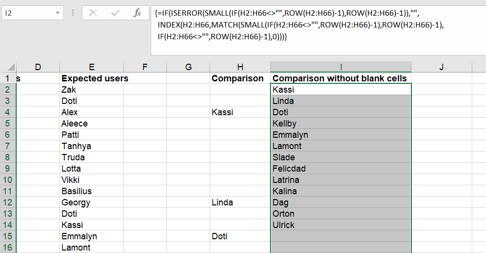
You can use this array formula for your cases by replacing H2:H66 with your range.