The VLOOKUP function looks up only one value. And what if you want to return a result that matches multiple criteria? Check out the following workaround.
How to VLOOKUP for multiple criteria
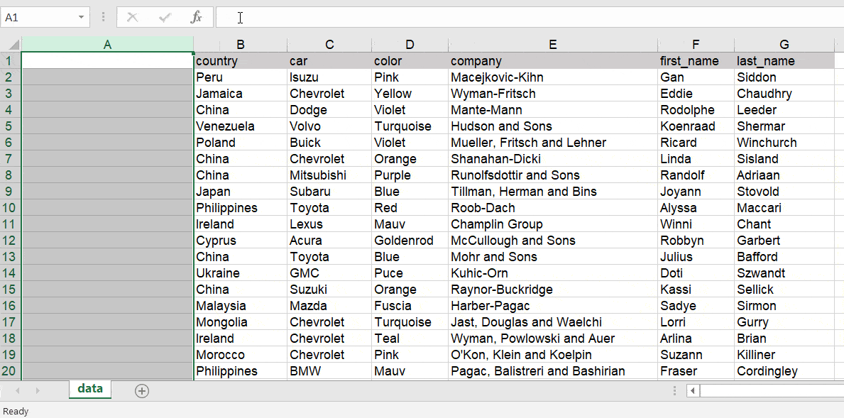
We imported a dataset from Google Sheets to Excel using Coupler.io, a solution for automatic data exports from multiple apps and sources. Read more about Microsoft Excel integrations for data export on a schedule.
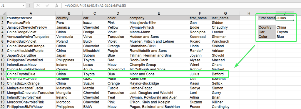
Our purpose is to look up the first name of a user by the following criteria:
- Country – China
- Car – Toyota
- Color – Blue
You can’t specify more than one lookup value in a VLOOKUP formula, so we’ll need to use a workaround, which consists of two steps:
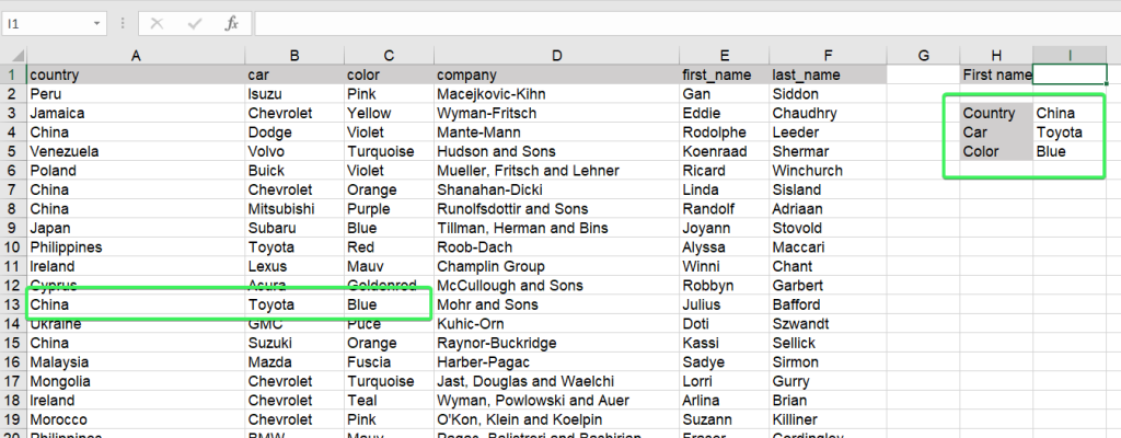
- Step1: Create a separate column where we will create unique lookup values by merging our lookup criteria – country, car, and color – “ChinaToyotaBlue“.
- Step2: We’ll use this lookup value in a VLOOKUP formula to return a matching value.
Step1: Create a column with unique lookup values made of two lookup criteria
- Insert a column to the left of your dataset like this. Select the entire column, insert the following formula to the formula bar and press Ctrl+Shift+Enter for Windows (Command+Return for Mac) – This will apply an array formula in Excel:
=B1:B100&C1:C1000&D1:D100
This formula will merge values from columns B, C, and D in the specified array.
Step2: VLOOKUP formula for multiple values
Now we can use a VLOOKUP formula, which will contain multiple lookup criteria merged into one lookup value:
=VLOOKUP((J3&J4&J5),A2:G101,6,FALSE)
(J3&J4&J5)– a lookup value based on the formula, which merges criteria from cells J3 (China), J4 (Toyota), and J5 (Blue).A2:G101– the range to look up6– the column to return the matching values from