Compared to simple spreadsheet applications like Google Sheets, BigQuery provides a framework and advanced query mechanism to help you perform deeper analysis on your data and extract valuable insights. BigQuery’s query mechanism is powered by Structured Query Language (SQL), which is a programming language created explicitly for database management systems and is particularly useful in handling structured data.
Even if you are not already familiar with SQL, it’s not rocket science. The learning curve is not that steep, and you can master SQL with some dedication and effort. In this tutorial, you will learn the fundamentals of SQL and BigQuery so you can get started with the proper foundation.
Introduction to Google BigQuery SQL
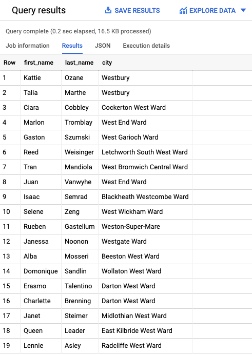
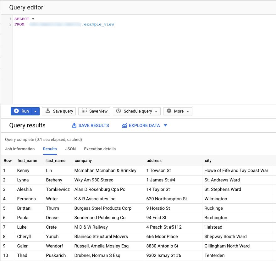
Besides the performance and scalability features, what makes BigQuery so popular is its ease of use. As Google BigQuery is using SQL as its query language, which is the standard query language for many popular database and data warehouse systems, database developers and analysts are already familiar with it. Here is an example of an SQL query along with the returned results, right from BigQuery:
SELECT
  first_name,
  last_name,
  city
FROM
  `project.dataset.example`
WHERE
  city LIKE '%West%'
Check out this SQL video tutorial for beginners made by Railsware Product Academy.
What types of SQL is BigQuery using?
When BigQuery was first introduced, all executed queries were using a non-standard SQL dialect known as BigQuery SQL. After the new version of BigQuery was released (BigQuery 2.0), the Standard SQL was supported, and BigQuery SQL was renamed Legacy SQL. Currently, BigQuery supports both types (or dialects) of SQL: Standard SQL and Legacy SQL. You can use the dialect of your choice without any performance issues.
Difference between Standard and Legacy SQL
The main difference between Standard SQL and Legacy SQL lies in their supported functions and query structure. Moreover, Standard SQL complies with the SQL 2011 standard, and has extensions that support querying nested and repeated data, provide data types to handle custom fields such as ARRAY and STRUCT, and allow complex joins of different data. This is the main reason that Google recommends Standard SQL as the query syntax.
Below is a quick example on how we can calculate the number of distinct users in both dialects. As you can see, while Legacy SQL requires a function to calculate the result, Standard SQL is more flexible in terms of syntax.
#legacySQL
SELECT EXACT_COUNT_DISTINCT(user)
FROM V;
#standardSQL
SELECT COUNT(DISTINCT user)
FROM V;
How to switch to Standard SQL
For new projects, Google is using Standard SQL in Query settings by default, so you don’t have to do anything further. For existing projects, you can use a query prefix on the query console to define the dialect. To do that, you can just write:
- #legacySQL – to run the query using Legacy SQL
- #standardSQL – to run the query using Standard SQL
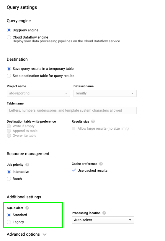
In the Cloud Console, when you use a query prefix, the SQL dialect option is disabled in the Query settings. If you want to change the dialect using the Query settings, you can:
- Open BigQuery Console.
- Click “More” > “Query Settings”.
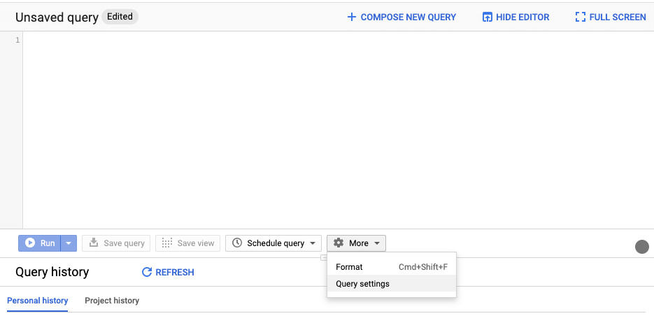
- Select the SQL dialect of preference.
What is BigQuery BI Engine?
While BigQuery is great for storage and business analysis purposes, there are cases where speed requirements are high, so the responses must be faster even than a couple of seconds. This is where the BigQuery BI Engine comes in. BigQuery BI Engine is a fast, in-memory analysis service with which you can analyze data stored in BigQuery with sub-second query response time and high concurrency.
In order to enable BI Engine for your BigQuery project, you can:
- Open BigQuery Admin Console BI Engine.
- Click “Create reservation”.
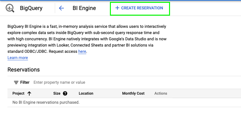
- Verify your project name, select your location, and adjust the slider so you can give the amount of memory needed for your calculations.
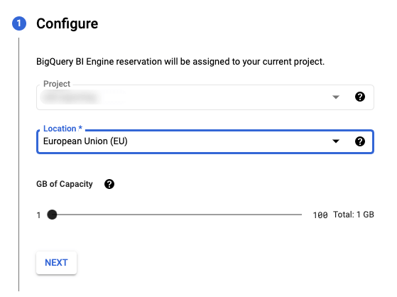
- Click “NEXT” and then “Create” to create your reservation for this project and enable the BI Engine.
You can then connect popular BI Tools, for example, connect BigQuery to Tableau, Google Data Studio, Looker or Power BI to accelerate data exploration and analysis. Just like the BigQuery service overall, the BigQuery BI Engine comes with a free tier, but depending on usage, you may have an additional cost to the BigQuery.
BigQuery SQL Syntax
In order to fetch data from BigQuery tables and analyze them you will have to write query statements in SQL to scan one or more tables and return the computed result rows. “What’s a query statement?” you may ask. Let’s start by explaining the basic terminology around SQL:
- Query expression: a set of instructions that tell the database what action should perform.
- Query statement: one or many query expressions executed by the database system all together.
- Clause: a specific command that forms a query expression. Popular SQL clauses include
SELECT,FROM,WHERE, andGROUP BY. - Function: a predefined set of clauses that perform a complex action. Examples of SQL functions are
COUNT,SUM, and so on. - Operation: when a specific query statement is executed and the database system interacts with the data. The available operations a system can perform are
CREATE,READ,UPDATE, andDELETE. - Record: a set of information in structured data. If we visualize the data in a tabular format, a record can also be described as a row.
- Column: a piece of information that belongs to a record just like when we read the data in a tabular format.
Below we’ll show you the query syntax for SQL queries in BigQuery. When writing a query expression, we essentially write multiple clauses. The clauses must appear with the following sequence:
query_expr:
        SELECT ...
	FROM ...
	WHERE ...
	GROUP BY ...
	HAVING ...
	ORDER BY...
In the following sections, we’ll apply everything on a sample dataset to have a better visual representation of the queried table along with the computed result rows. If you do not have any data loaded to BigQuery yet, you can use Coupler.io to import your data from different sources or Google Sheets in a quick and easy way. Just export your data and, by following a really simple flow, you’ll have everything loaded from Google Sheets to BigQuery in a matter of minutes.
BigQuery SQL Syntax: SELECT list
The SELECT list defines the set of columns that the query should return. The items within the SELECT list can refer to columns in any of the items within the FROM clause. Each item in the SELECT list can be any of the below:
SELECT *
Often referred to as the SELECT star, this expression returns all of the corresponding columns from each item of the FROM list. Let’s say we have a table called CLIENTS that contains the first name, surname, email, and telephone number for each client. After executing the query, these results are returned:
SELECT * FROM `CLIENTS`;
SELECT expression
All the items in the SELECT list can be expressions. These expressions can describe a single column and produce one column output. For example, using the same CLIENTS table:
SELECT first_name, email FROM `CLIENTS`;
BigQuery SQL Syntax: FROM clause
The FROM clause defines the source from which we’ll select the data. This can be a single table or multiple tables at once, but we have to also define how these tables are joined together. We’ll talk about the JOIN operation in the next subsection. In the meantime, below you can find a couple of ways to use the FROM clause if we want to query data from the CLIENTS table specifying the table if it’s unique, the dataset and the table if the table name is unique within the dataset and the project, or dataset and table if the table name is unique within the project:
SELECT * FROM `CLIENTS`;
SELECT * FROM `dataset.CLIENTS`;
SELECT * FROM `project.dataset.CLIENTS`;
Specifying the dataset or project is also extremely convenient when you are managing multiple projects and datasets and you need to be specific on which project or dataset to use.
BigQuery SQL Syntax: JOIN operation
The JOIN operations are maybe one of the most important operations in SQL as they can help you combine data from multiple tables or views. There are several types of joins and we’ll go through each one of them below:
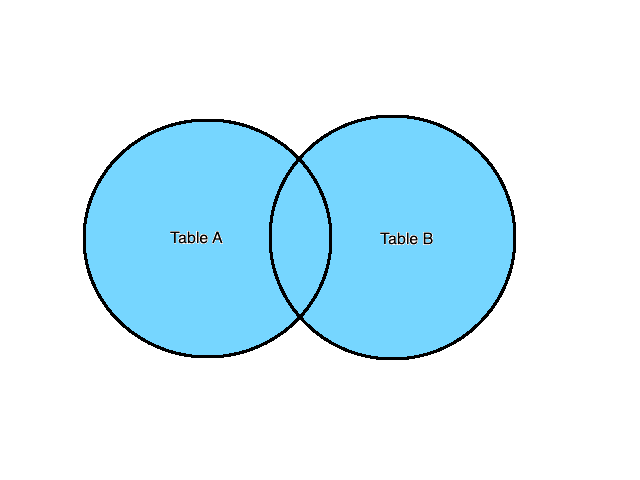
INNER JOIN (or just JOIN)
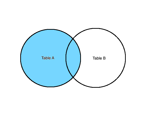
INNER JOIN or simply JOIN is the operation that effectively calculates the Cartesian product of the two tables based on a common value. Essentially, JOIN selects all records that have matching values in both tables. A visual representation of the INNER JOIN is:

Let’s see how we can use JOIN to combine data from the below two tables:
Table A
| a | b |
|---|---|
| 1 | aaa |
| 2 | bbb |
| 3 | ccc |
Table B
| c | d |
|---|---|
| 1 | fff |
| 2 | ccc |
| 4 | ggg |
If we use the below query, we’ll end up with the final table containing all the data and columns that share the same value in column a (from Table A) and column c (from Table B) as we define with the ON parameter.
SELECT *
FROM A
INNER JOIN B
      ON A.a = B.c
| a | b | c | d |
|---|---|---|---|
| 1 | aaa | 1 | fff |
| 2 | bbb | 2 | ccc |
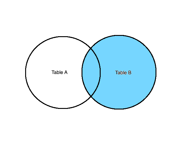
CROSS JOIN
Opposed to the INNER JOIN, the CROSS JOIN operation will return the Cartesian product of the two tables regardless of a common value. A visual representation is:

We will use CROSS JOIN to combine data from the below two tables:
Table A
| a | b |
|---|---|
| 1 | aaa |
| 2 | bbb |
Table B
| c | d |
|---|---|
| 1 | fff |
| 3 | ccc |
We can use the below query and we’ll end up with the final table containing all the data from both tables. As you can see, there is no ON parameter as the tables don’t need to share a common value.
SELECT *
FROM A
CROSS JOIN B
| a | b | c | d |
|---|---|---|---|
| 1 | aaa | 1 | fff |
| 1 | aaa | 3 | ccc |
| 2 | bbb | 1 | fff |
| 2 | bbb | 3 | ccc |
FULL JOIN (or FULL OUTER JOIN)
The FULL JOIN or FULL OUTER JOIN returns all records when there is a match in the left (Table A) or right (Table B) table records. Usually, FULL OUTER JOIN can return very large result sets. This is similar to the CROSS JOIN operation, except we have a matching condition to join rows (if they exist). Let’s see a visual representation and the usage of FULL OUTER JOIN in action:
We will use FULL OUTER JOIN to combine data from the below two tables:
Table A
| a | b |
|---|---|
| 1 | aaa |
| 2 | bbb |
Table B
| c | d |
|---|---|
| 1 | fff |
| 3 | ccc |
We can use the following query and we’ll end up with the final table containing all the data from both tables:
SELECT *
FROM A
FULL OUTER JOIN B
      ON A.a = B.c
| a | b | c | d |
|---|---|---|---|
| 1 | aaa | 1 | fff |
| 2 | bbb | NULL | NULL |
NULL | NULL | 3 | ccc |
LEFT JOIN (or LEFT OUTER JOIN)
LEFT JOIN or LEFT OUTER JOIN operation always returns all the items from the left item in the FROM clause even if no rows in the right item satisfy the join predicate. This is different from the FULL OUTER JOIN as the rows that only exist in the second table are not returned. Let’s see this type of join in action:
Using the same tables as before, we can calculate the LEFT JOIN like this:
Table A
| a | b |
|---|---|
| 1 | aaa |
| 2 | bbb |
Table B
| c | d |
|---|---|
| 1 | fff |
| 3 | ccc |
SELECT *
FROM A
LEFT OUTER JOIN B
      ON A.a = B.c
| a | b | c | d |
|---|---|---|---|
| 1 | aaa | 1 | fff |
| 2 | bbb | NULL | NULL |
RIGHT JOIN (or RIGHT OUTER JOIN)
Similar to the LEFT JOIN, the RIGHT JOIN (or RIGHT OUTER JOIN) operation behaves the same way, only it focuses on the right item of the FROM list. Let’s see that in action:
Calculating the RIGHT JOIN on the below tables returns these results:
Table A
| a | b |
|---|---|
| 1 | aaa |
| 2 | bbb |
Table B
| c | d |
|---|---|
| 1 | fff |
| 3 | ccc |
SELECT *
FROM A
RIGHT OUTER JOIN B
       ON A.a = B.c
| a | b | c | d |
|---|---|---|---|
| 1 | aaa | 1 | fff |
NULL | NULL | 3 | ccc |
BigQuery SQL Syntax: WHERE clause
The WHERE clause is as simple as it is important for the queries. Essentially, this clause filters the results of the FROM clause. The syntax follows this structure:
SELECT *
FROM `CLIENTS`
WHERE bool_expression
Only rows whose bool_expression evaluates to TRUE are included. Rows whose bool_expression evaluates to NULL or FALSE are discarded. For example, let’s say we have this table:
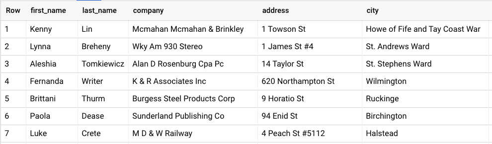
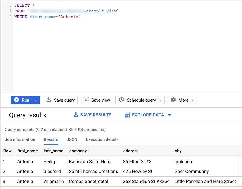
We can use the WHERE clause to filter and keep only the people named “Antonio”. Let’s see this query:
SELECT *
FROM `CLIENTS`
WHERE first_name=”Antonio”
This will return only the rows that match this condition, so the result set will look like this:
BigQuery SQL Syntax: GROUP BY clause
When we’re analyzing data, we usually perform calculations on them to get better insights. This is achieved by using aggregation functions like counting the results or summing some metrics. We’ll talk about aggregation functions in the following subsection, but when we want to aggregate metrics, it’s important to define which columns will be aggregated and which will not be.
The GROUP BY clause groups together rows in a table with non-distinct values for the expression in the GROUP BY clause. Let’s see an example:
SELECT first_name, COUNT(company) AS number_of_companies
FROM `CLIENTS`
GROUP BY first_name
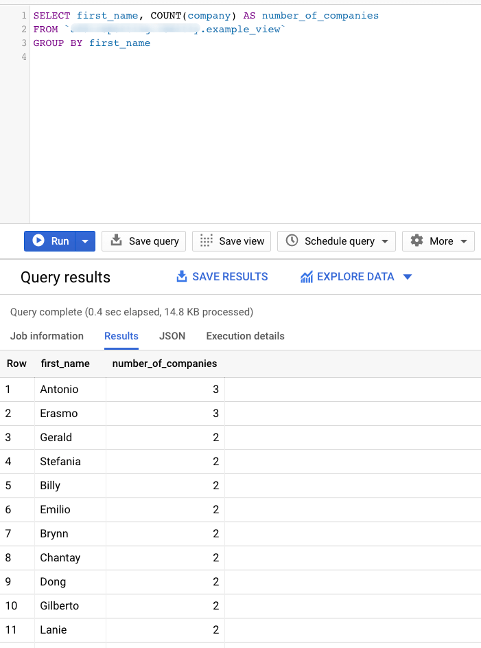
The above query will count all the different companies of a person with the same first name works. This is achieved by defining that all purchases must be summed and grouped by every distinct last name.
BigQuery SQL Syntax: HAVING clause
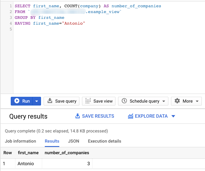
The HAVING clause is similar to the WHERE clause, only it focuses on the results produced by the GROUP BY clause. If aggregation is present, the HAVING clause is evaluated once for every aggregated row in the result set. For example, if we want to return the number of different companies any person named “Antonio” works we can use this query:
SELECT first_name, COUNT(company) AS number_of_companies
FROM `CLIENTS`
GROUP BY first_name
HAVING first_name="Antonio"
BigQuery SQL Syntax: ORDER BY clause
Using the ORDER BY clause, we can define exactly how the result set will be ordered and the priority. The ORDER BY clause comes at the end of each query to sort the final result set. For example, if we want to sort the result set shown in the previous subsection based on the First Name in ascending order, we can do this:
SELECT first_name, COUNT(company) AS number_of_companies
FROM `CLIENTS`
GROUP BY first_name
HAVING first_name="Antonio"
ORDER BY first_name ASC
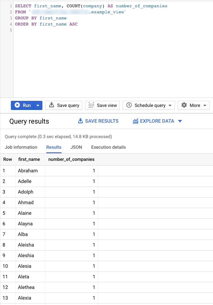
If the ORDER BY clause is not present, the order of the results of a query is not defined.
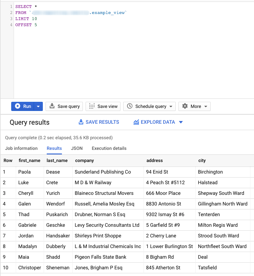
BigQuery SQL Syntax: LIMIT & OFFSET clauses
Another two great and useful clauses are LIMIT and OFFSET. Using LIMIT followed by a positive integer number, we can specify the number of rows that will be returned from the query. LIMIT 0 returns 0 rows.
OFFSET specified a non-negative number of rows to skip before applying LIMIT. These clauses accept only literal or parameter values. Below is an example showing how we can return 10 rows after we skip the first 5 of the result set.
SELECT *
FROM `CLIENTS`
LIMIT 10
OFFSET 5;
BigQuery SQL Syntax: WITH clause
The WITH clause is a great way to temporarily store a subquery and use it each time it is needed. A subquery is a complete query expression within a parenthesis. This means that is evaluated first, and the results can be used by the query expression out of the parenthesis.
The WITH clause contains one or more named subqueries that execute every time a subsequent SELECT statement references them.
WITH SubQ1 AS (
  SELECT first_name
  FROM CLIENTS
)

SELECT *
FROM subQ1
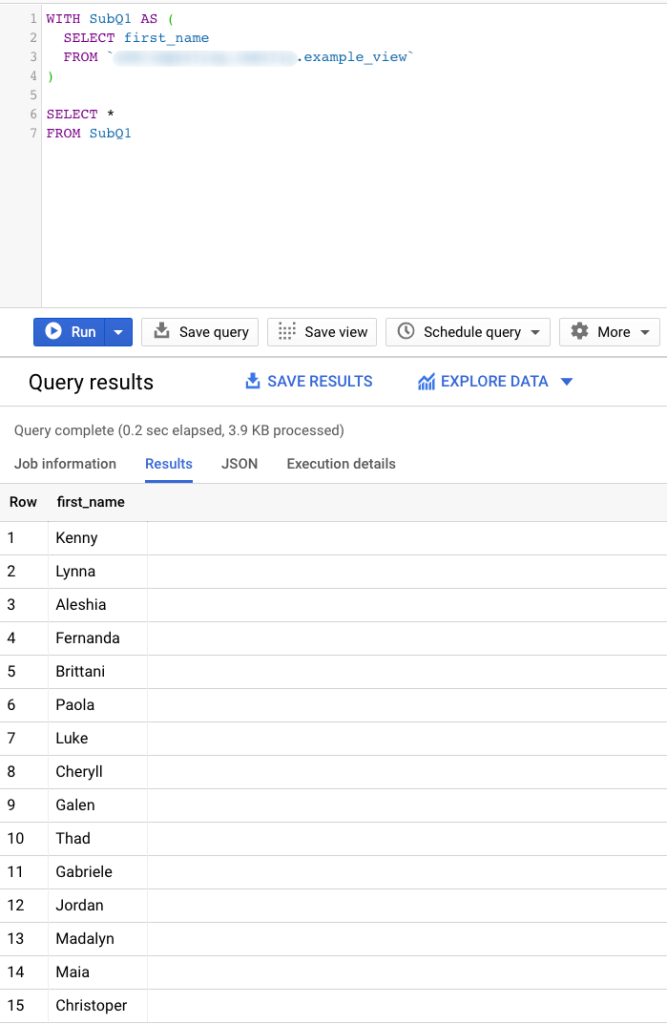
In the above query, we store a simple query and we name it as “subQ1”, and then we can reference this in a FROM clause just like every other table.
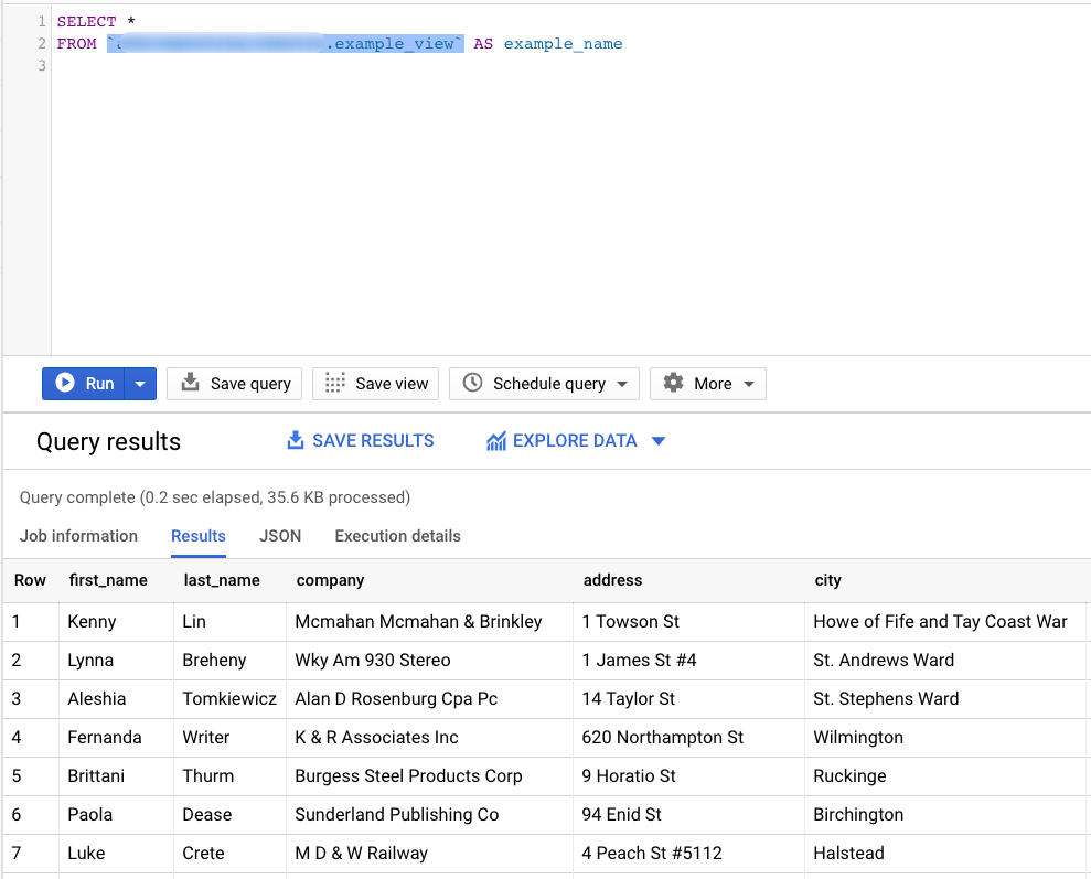
BigQuery SQL Syntax: Using aliases
A great way to optimize your code and make it more readable is by using aliases. An alias is a temporary name given to a table, column, or expression present in a query. In the previous subsection, we introduced a subquery called “subQ1”. This is an alias that allows us to reference a whole query with a single name. Moreover, tables can have big names (e.g. whether_conditions_uk_2016), which is not ideal when we want to reference them. An alias can help us create a shorter name to use in our queries.
An example of table alias is shown below where we apply an alias to the CLIENTS table to call it “example_name”:
SELECT *
FROM whether_conditions_uk_2016 AS example_name
BigQuery SQL Important Functions
Now that we have seen how to construct a query in BigQuery SQL and what the syntax is, it’s important to see core functions that you can use to power up your analytics capabilities. We’ll discuss several types of functions, and we’ll show the most popular and useful ones that will help you extract core insights from your data.
BigQuery SQL Functions: Aggregate functions
Aggregate functions are maybe the most used type of SQL function. An aggregate function summarizes the rows of a group into a single value. Let’s see the most common ones along with some examples:
AVG
The AVG function takes any numeric input type and returns the average or NaN if the input contains not a number value. Let’s see a quick example using the below dataset:
| name | age |
|---|---|
| John Doe | 37 |
| John Davis | 42 |
| Jessie Cole | 19 |
| Jack Delaney | 74 |
If we want to find the average age of our group, we can use this query:
SELECT AVG(age)
FROM CLIENTS AS avg_age
The result set will look like this:
| avg_age |
|---|
| 23.25 |
COUNT
The COUNT function takes any row input and returns the total number of rows in the input. Let’s see a quick example using the below dataset:
| name | age |
|---|---|
| John Doe | 37 |
| John Davis | 42 |
| Jessie Cole | 19 |
| Jack Delaney | 74 |
If we want to find the total number of people in our group, we can use this query:
SELECT COUNT(name)
FROM CLIENTS AS number_of_people
The result set will look like this:
| number_of_people |
|---|
| 4 |
MAX
The MAX function takes any row input and returns the maximum value of non-NULL rows in the input. Let’s see a quick example using the below dataset:
| name | age |
|---|---|
| John Doe | 37 |
| John Davis | 42 |
| Jessie Cole | 19 |
| Jack Delaney | 74 |
If we want to find the oldest age in our group, we can use this query:
SELECT MAX(age)
FROM CLIENTS AS max_age
The result set will look like this:
| max_age |
|---|
| 74 |
MIN
Opposed to the MAX function, the MIN function takes any row input and returns the minimum value of non-NULL rows in the input. Using the below dataset:
| name | age |
|---|---|
| John Doe | 37 |
| John Davis | 42 |
| Jessie Cole | 19 |
| Jack Delaney | 74 |
If we want to find the youngest age in our group, we can use this query:
SELECT MIN(age)
FROM CLIENTS AS min_age
The result set will look like this:
| min_age |
|---|
| 19 |
SUM
Last but not least, the most popular aggregate function is SUM. This function takes any numeric non-null row input and returns the sum of the values. We can use the below dataset:
| name | purchases |
|---|---|
| John Doe | 12 |
| John Davis | 1 |
| Jessie Cole | 22 |
| Jack Delaney | 44 |
If we want to find the total number of purchases, we can use this query:
SELECT SUM(purchases)
FROM CLIENTS AS total_purchases
The result set will look like this:
| total_purchases |
|---|
| 79 |
BigQuery SQL Functions: Mathematical functions
Mathematical functions come in handy when you want to quickly calculate results between two or more numbers. Essentially, all mathematical functions have the following behaviors:
- They return NULL if any of the input parameters appears to be blank.
- They return NaN if any of the arguments are not a number.
Let’s take a closer look at some of the most popular ones:
RAND
RAND generates a pseudo-random value of type FLOAT64 in the range of (0, 1), inclusive of 0 and exclusive of 1. It doesn’t need any arguments, and you can use it like this:
RAND()
SQRT
SQRT computes the square root of the input X. It generates an error if X is less than 0, and below is a quick example of such usage:
SQRT(X)
POW
POW or POWER returns the value of input X raised to the power of input Y.
POW(X, Y)
DIV
DIV is the simple division between two integers. Returns the result of integer division of input X by input Y. Division by zero returns an error and division by -1 may overflow.
DIV(X, Y)
SAFE_DIVIDE
If you need to avoid the error in your query (e.g. if you divide by zero), you can use SAFE_DIVIDE. This function is equivalent to the DIV but returns NULL if an error occurs, such as a division by zero error.
SAFE_DIVIDE(X, Y)
ROUND
ROUND is responsible to round the input X to the nearest integer. If a second input N is present, ROUND rounds X to N decimal places after the decimal point. If N is negative, then it will round off digits to the left of the decimal points.
ROUND(X, [, N])
CEIL
If you want to specify the rounding rules and always round down to the largest integral value of the input X, then you should use CEIL or CEILING. This function rounds the input X to the largest integral value that is not greater than X.
CEIL(X)
FLOOR
Opposed to CEIL, if you want to round to the smallest integral value of the input X that is not less than X, you should use the FLOOR function.
FLOOR(X)
BigQuery SQL Functions: String functions
String functions are really useful for manipulating text fields. These string functions work on two different values: STRING and BYTES data types. STRING values must be well-formed UTF-8. Let’s see some of the most useful string functions.
CONCAT
CONCAT concatenates one or more values into a single result. All values must be BYTES or data types that can be cast to STRING.
SELECT CONCAT("Hello", " ", "World") AS concatenated_string
| concatenated_string |
|---|
| Hello World |
ENDS_WITH
ENDS_WITH takes two STRING or BYTES values and returns TRUE if the second value is a suffix of the first one, otherwise it returns FALSE. Let’s see an example applying this function in the below dataset.
| fruit |
|---|
| Banana |
| Apple |
| Orange |
| Apricot |
SELECT ENDS_WITH(fruit, "e") AS example
FROM FRUITS
Based on the above dataset and using the query, we end up with this result set:
| example |
|---|
| FALSE |
| TRUE |
| TRUE |
| FALSE |
STARTS_WITH
Similarly, STARTS_WITH takes two STRING or BYTES values and returns TRUE if the second value is a prefix of the first one, otherwise it returns FALSE. An identical example if we use the below dataset would be:
| fruit |
|---|
| Banana |
| Apple |
| Orange |
| Apricot |
SELECT STARTS_WITH(fruit, "A") AS example
FROM FRUITS
Based on the above dataset and using the query, we end up with this result set:
| example |
|---|
| FALSE |
| TRUE |
| FALSE |
| TRUE |
LOWER
Another simple yet useful string function is LOWER. It takes a STRING or BYTES input and transforms it to lowercase. For example:
SELECT LOWER("Hello") AS lowered_string
| lowered_string |
|---|
| hello |
UPPER
Similar to the LOWER function is the UPPER, but instead of transforming the input to lowercase, it transforms it to uppercase.
SELECT UPPER("Hello") AS uppered_string
| uppered_string |
|---|
| HELLO |
REGEXP_CONTAINS
REGEXP_CONTAINS returns TRUE if the value is a partial match for the regular expression. If the regular expression argument is invalid, the function returns an error. Let’s see an example using the below dataset:
| test@example.com |
| another_test@example.com |
| wow.test.com |
| example.com/test@ |
We can use the REGEXP_CONTAINS to verify whether the email is valid or not, as shown below:
SELECT
  email,
  REGEXP_CONTAINS(email, "@[a-zA-Z0-9-]+\.[a-zA-Z0-9-.]+") AS is_valid
FROM EMAILS
| is_valid |
|---|
| TRUE |
| TRUE |
| FALSE |
| FALSE |
REGEXP_EXTRACT
A great use of regular expression string function is if we want to extract a certain part of a string. REGEXP_EXTRACT returns the substring in input value that matches the regular expression and NULL if there is no match. Using the below dataset, we can extract the first part of the email address using the following query:
| test@example.com |
| another_test@example.com |
SELECT
  REGEXP_EXTRACT(email, r"^[a-zA-Z0-9_.+-]+") AS user_name
FROM EMAILS
| user_name |
|---|
| test |
| another_test |
REGEXP_REPLACE
REGEXP_REPLACE returns a string where all substrings of the input value that match the input regular expression are replaced with the replacement value. Let’s see an example where we replace every “pie” occurrence with “jam”:
SELECT
  REGEXP_REPLACE("Apple pie or Cherry pie?", "pie", "jam") AS re
| re |
|---|
| Apple jam or Cherry jam? |
REPLACE
Similarly to the REGEXP_REPLACE, but without the use of RegEx, is the REPLACE function. It replaces all occurrences of the “from” input value with the “to” input value in the original input value. If the “from” input value is empty, no replacement is made.
SELECT REPLACE("Apple pie", "pie", "jam") AS re
| re |
|---|
| Apple jam |
SPLIT
SPLIT splits the input value using the given delimiter. For STRING input value, the default delimiter is the comma. Splitting an empty STRING input returns an ARRAY with a single empty STRING.
SELECT SPLIT("Apple pie or not?", " ") AS re
| re |
|---|
| [Apple, pie, or, not?] |
SUBSTR
Last but not least, SUBSTR returns a substring of the supplied STRING or BYTES value. The position argument is an integer specifying the starting position of the substring. If the position is negative, the function will start counting from the end of the input value, with -1 indicating the last character. For example:
SELECT SUBSTR("apple", 3) AS substring
| re |
|---|
| ple |
BigQuery SQL Functions: Array functions
Array functions allow you to manipulate an array and its elements. In BigQuery, an array is an ordered list consisting of zero or more values of the same data type. You can create an array to group similar information together rather than having them split into columns, and then you can use them as needed. Below you will learn how to handle arrays using array functions.
ARRAY
The ARRAY function returns an array with one element for each row in a subquery. For example, the below query will generate a final array with all the elements of the subquery.
SELECT ARRAY
  (SELECT "a" UNION ALL
   SELECT "b" UNION ALL
   SELECT "c") AS generated_array
| generated_array |
|---|
| [“a”, “b”, “c”] |
ARRAY_CONCAT
ARRAY_CONCAT concatenates one or more arrays with the same element type into a single array.
SELECT ARRAY_CONCAT(["a", "b"], ["c", "d"], ["e", "f"]) AS starting_alphabet
| starting_alphabet |
|---|
| [“a”, “b”, “c”, “d”, “e”, “f”] |
ARRAY_LENGTH
ARRAY_LENGTH returns the size of the array and zero if the array is empty.
SELECT ARRAY_LENGTH(["a", "b"]) AS array_length
| array_length |
|---|
| 2 |
ARRAY_TO_STRING
ARRAY_TO_STRING transforms arrays to strings by concatenating all of the elements. This function takes an array and a concatenation value as an input, like this:
SELECT ARRAY_TO_STRING(["a", "b"], "--") AS array_to_string
| array_to_string |
|---|
| a–b |
BigQuery SQL Functions: Date functions
Date functions are great when you need to handle dates in your dataset. Let’s see the most common date functions that BigQuery offers:
CURRENT_DATE
CURRENT_DATE returns the current date for the specified or the default timezone.
SELECT CURRENT_DATE() AS today;
| today |
|---|
| 2021-05-10 |
EXTRACT
When you’re using EXTRACT, providing a DATE field allows you to extract a specific part of the date. The provided part must be any of the below:
- DAYOFWEEK: value from 1 to 7. Sunday is the first day of the week.
- DAY: value from 1 to 31 depending on the month.
- DAYOFYEAR: value from 1 to 365 (or 366 for leap years).
- WEEK: value from 0 to 53. Sunday is the first day of the week. For the dates prior to the first Sunday of the year, the function will return 0.
- WEEK(<WEEKDAY>): value from 0 to 53. The specified WEEKDAY is the first day for the week. For the dates prior to the first WEEKDAY of the year, the function will return 0.
- ISOWEEK: value from 1 to 53 using the ISO 8601 week boundaries. Monday is the first day of the ISOWEEK. The first ISOWEEK of each ISO year begins on the Monday before the first Thursday of the Gregorian calendar year.
- MONTH: value from 1 to 12. January is the first month of the year.
- QUARTER: value from 1 to 4.
- YEAR: year value in the format YYYY.
- ISOYEAR: year value using the ISO 8601 format boundaries.
Let’s see a quick example on how to use the EXTRACT function:
SELECT EXTRACT(MONTH FROM DATE '2021-05-01') AS the_day
| the_day |
|---|
| 05 |
DATE
The DATE function is responsible for constructing a DATE field from integer values representing the year, month, and day.
SELECT DATE(2018, 11, 23) AS specific_date
| specific_date |
|---|
| 2018-11-23 |
DATE_ADD
DATE_ADD adds a specific time interval to an input DATE value. The interval must be provided as an input and can be any of the below:
- DAY
- WEEK
- MONTH
- QUARTER
- YEAR
You can use the DATE_ADD function like this:
SELECT DATE_ADD(DATE "2018-11-23", INTERVAL 2 DAY) AS two_days_later
| two_days_later |
|---|
| 2018-11-25 |
DATE_SUB
DATE_SUB works similarly to the DATE_ADD, but instead of adding a specific time interval to the input DATE value, it subtracts the interval from it. For example:
SELECT DATE_SUB(DATE "2018-11-23", INTERVAL 2 DAY) AS two_days_earlier
| two_days_earlier |
|---|
| 2018-11-21 |
DATE_DIFF
DATE_DIFF calculates the number of whole specified intervals between two DATE objects.
SELECT DATE_DIFF(DATE '2018-11-25', DATE '2018-11-29', DAY) AS day_difference
| day_difference |
|---|
| 4 |
FORMAT_DATE
FORMAT_DATE formats the input DATE field to the specified format string. The supported format elements for a DATE field can be found here.
SELECT FORMAT_DATE("%b %d, %Y", DATE "2018-11-22") AS new_format
| new_format |
|---|
| Nov 22, 2018 |
PARSE_DATE
PARSE_DATE is maybe the most simple function between date functions, but also the most used one. PARSE_DATE converts a string representation of date to a DATE object. In order for the PARSE_DATE to work, the two inputs (format string and date string) have to match.
For example, the below query will work because the two inputs match:
SELECT PARSE_DATE("%b %e %Y", "Dec 25 2018")
On the other hand, the following query will not work because the two inputs do not match:
SELECT PARSE_DATE("%b %e %Y", "Sunday May 09 2021")
BigQuery SQL Functions: Datetime functions
Besides DATE fields, BigQuery SQL also supports DATETIME functions that behave similarly to the DATE functions, but for DATETIME fields. A DATETIME object represents a date and time as it might be displayed on a calendar or clock, independent of time zone. Let’s see the functions:
CURRENT_DATETIME
CURRENT_DATETIME returns the current date and time for the specified or the default time zone.
SELECT CURRENT_DATETIME() AS today
| today |
|---|
| 2021-05-10T10:38:47.046465 |
DATETIME
The DATETIME function is responsible to construct a DATETIME field from integer values representing the year, month and day, hour, minute and second.
SELECT DATE(2018, 11, 23, 10, 21, 44) AS specific_date
| specific_date |
|---|
| 2018-11-23T10:21:44 |
EXTRACT
When you’re using EXTRACT and provide a DATETIME field, it allows you to extract a specific part of the date/time value. The provided part must be any of the below:
- MICROSECOND
- MILLISECOND
- SECOND
- MINUTE
- HOUR
- DAYOFWEEK
- DAY
- DAYOFYEAR
- WEEK
- WEEK(<WEEKDAY>)
- ISOWEEK
- MONTH
- QUARTER
- YEAR
- ISOYEAR
Let’s see a quick example on how to use the EXTRACT function:
SELECT EXTRACT(HOUR FROM DATETIME(2021, 05, 01, 10, 23, 11)) AS hour
| hour |
|---|
| 10 |
DATETIME_ADD
DATETIME_ADD adds a specific time interval to an input DATETIME value. The interval must be provided as an input and can be any of the below:
- MICROSECOND
- MILLISECOND
- SECOND
- MINUTE
- HOUR
- DAY
- WEEK
- MONTH
- QUARTER
- YEAR
You can use the DATETIME_ADD function as shown below:
SELECT DATETIME_ADD(DATETIME "2018-11-23 15:30:02", INTERVAL 10 MINUTE) AS ten_minutes_later
| ten_minutes_later |
|---|
| 2018-11-23T15:40:02 |
DATETIME_SUB
DATETIME_SUB works similarly to the DATETIME_ADD function, except instead of adding a specific time interval to the input DATETIME value, it subtracts the interval from it. For example:
SELECT DATE_SUB(DATE "2018-11-23 15:30:02", INTERVAL 2 HOURS) AS two_hours_earlier
| two_hours_earlier |
|---|
| 2018-11-23T13:30:02 |
DATETIME_DIFF
DATETIME_DIFF calculates the number of whole specified intervals between two DATE objects.
SELECT DATE_DIFF(DATE '2018-11-25 14:24:44', DATETIME '2018-11-25 17:22:42', HOUR) AS hour_difference
| hour_difference |
|---|
| 3 |
FORMAT_DATETIME
FORMAT_DATETIME formats the input DATETIME field to the specified format string.
SELECT FORMAT_DATETIME("%b %d, %Y", DATETIME "2018-11-22 15:30:22") AS new_format
| new_format |
|---|
| Nov 22, 2018 |
BigQuery SQL Functions: Time functions
BigQuery SQL also supports time functions to help you handle TIME objects. Let’s see the most important ones:
CURRENT_TIME
CURRENT_TIME returns the current time for the specified or the default time zone.
SELECT CURRENT_TIME() AS now
| now |
|---|
| 10:38:47.046465 |
TIME
The TIME function constructs a TIME field value from integer values representing the hour, minute and second.
SELECT DATE(10, 21, 44) as specific_time
| specific_time |
|---|
| 10:21:44 |
EXTRACT
When you’re using EXTRACT and provide a TIME field, it allows you to extract a specific part of the time value. The provided part must be any of the below:
- MICROSECOND
- MILLISECOND
- SECOND
- MINUTE
- HOUR
Let’s see a quick example on how to use the EXTRACT function:
SELECT EXTRACT(HOUR FROM TIME "10:23:11") AS hour
| hour |
|---|
| 10 |
TIME_ADD
TIME_ADD adds a specific time interval to an input TIME value. The interval must be provided as an input and can be any of the below:
- MICROSECOND
- MILLISECOND
- SECOND
- MINUTE
- HOUR
You can use the TIME_ADD function, as shown below:
SELECT TIME_ADD(TIME "15:30:02", INTERVAL 10 MINUTE) AS ten_minutes_later
| ten_minutes_later |
|---|
| 15:40:02 |
TIME_SUB
TIME_SUB works similarly to the TIME_ADD, but instead of adding a specific time interval to the input TIME value, it subtracts the interval from it. For example:
SELECT TIME_SUB(TIME "15:30:02", INTERVAL 2 HOURS) AS two_hours_earlier
| two_hours_earlier |
|---|
| 13:30:02 |
TIME_DIFF
TIME_DIFF calculates the number of whole specified intervals between two TIME objects.
SELECT ΤΙΜΕ_DIFF(ΤΙΜΕ '14:24:44', TIME '17:22:42', HOUR) AS hour_difference
| hour_difference |
|---|
| 3 |
FORMAT_TIME
FORMAT_TIME formats the input TIME field to the specified format string.
SELECT FORMAT_TIME("%R", TIME "15:30:22") AS new_format
| new_format |
|---|
| 15:30 |
PARSE_TIME
PARSE_TIME converts a string representation of date to a TIME object. In order for the PARSE_TIME to work, the two inputs (format string and time string) have to match.
The example below will work because the two inputs match:
SELECT PARSE_TIME("%I:%M:%S", "17:30:02")
On the other hand, the following query will not work because the two inputs do not match:
SELECT PARSE_TIME("%I:%M", "17:30:02")
BigQuery SQL Functions: Timestamp functions
Besides the TIME functions, BigQuery SQL also supports TIMESTAMP functions. Bear in mind that these functions will return a runtime error if overflow occurs and the result values are bounded by the defined date and timestamp min and max values. Let’s jump right into the most popular functions and how you can use them:
CURRENT_TIMESTAMP
CURRENT_TIMESTAMP returns the current time for the specified or the default timezone.
SELECT CURRENT_TIMESTAMP() AS now
| now |
|---|
| 2021-05-10 21:23:11.120174 UTC |
TIMESTAMP
The TIMESTAMP function is responsible to construct a TIMESTAMP field from a string value representing the timestamp.
SELECT TIMESTAMP("2018-02-13 12:34:56+00") AS specific_date
| specific_date |
|---|
| 2018-02-13 12:34:56 UTC |
TIMESTAMP_ADD
TIMESTAMP_ADD adds a specific time interval to an input TIMESTAMP_ADD value. The interval must be provided as an input and can be any of the below:
- MICROSECOND
- MILLISECOND
- SECOND
- MINUTE
- HOUR
- DAY
You can use the TIMESTAMP_ADD function like this:
SELECT TIMESTAMP_ADD(TIMESTAMP("2018-11-23 15:30:02+00"), INTERVAL 10 MINUTE) AS ten_minutes_later
| ten_minutes_later |
|---|
| 2018-11-23 15:40:02 UTC |
TIMESTAMP_SUB
TIMESTAMP_SUB works similarly to the TIMESTAMP_ADD, but instead of adding a specific time interval to the input TIMESTAMP value, it subtracts the interval from it. For example:
SELECT TIMESTAMP_SUB(TIMESTAMP("2018-11-23 15:30:02+00"), INTERVAL 2 HOURS) AS two_hours_earlier
| two_hours_earlier |
|---|
| 2018-11-23 13:30:02 UTC |
TIMESTAMP_DIFF
TIMESTAMP_DIFF calculates the number of whole specified intervals between two TIMESTAMP objects.
SELECT TIMESTAMP_DIFF(TIMESTAMP("2018-11-25 14:24:44+00", TIMESTAMP("2018-11-25 17:22:42+00"), HOUR) AS hour_difference
| hour_difference |
|---|
| 3 |
FORMAT_TIMESTAMP
FORMAT_TIMESTAMP formats the input TIMESTAMP field to the specified format string.
SELECT FORMAT_TIMESTAMP("%b %d, %Y", TIMESTAMP "2018-11-22 15:30:22") AS new_format
| new_format |
|---|
| Nov 22, 2018 |
PARSE_TIMESTAMP
PARSE_TIMESTAMP converts a string representation of date to a TIMESTAMP object. In order for the PARSE_TIMESTAMP to work, the two inputs (format string and timestamp string) have to match.
For example, the below query will work because the two inputs match:
SELECT PARSE_TIMESTAMP("%b %e %I:%M:%S %Y", "Dec 25 07:44:32 2018")
On the other hand, the following query will not work because the two inputs do not match:
SELECT PARSE_TIMESTAMP("%a %b %e %I:%M:%S %Y", "Dec 25 07:44:32 2018")
TIMESTAMP_SECONDS
TIMESTAMP_SECONDS transforms the seconds since 1970-01-01 00:00:00 UTC and transforms them to a TIMESTAMP object.
SELECT TIMESTAMP_SECONDS(1589031996) AS timestamp_value
| timestamp_value |
|---|
| 2020-05-09 13:46:36 UTC |
TIMESTAMP_MILLIS
TIMESTAMP_MILLIS transforms the milliseconds since 1970-01-01 00:00:00 UTC and transforms them to a TIMESTAMP object.
SELECT TIMESTAMP_SECONDS(1589031996000) AS timestamp_value
| timestamp_value |
|---|
| 2020-05-09 13:46:36 UTC |
TIMESTAMP_MICROS
TIMESTAMP_MICROS transforms the microseconds since 1970-01-01 00:00:00 UTC and transforms them to a TIMESTAMP object.
SELECT TIMESTAMP_SECONDS(1589031996000000) AS timestamp_value
| timestamp_value |
|---|
| 2020-05-09 13:46:36 UTC |
Read our guide on Google BigQuery Datetime and Timestamp functions to learn more.
BigQuery SQL Functions: Operators
Operators exist to manipulate any number of data inputs and return a result. They are usually represented by a special character or keyword and do not use function call syntax. Below we’ll see the three most common operator types:
Arithmetic Operators
The arithmetic operators exist to manipulate two (or more) arithmetic inputs. All arithmetic operators accept input of numeric type X, and the result type has type X.
- Addition: X + Y
- Subtraction: X – Y
- Multiplication: X * Y
- Division: X / Y
Logical Operators
Logical operators exist to use three-valued logic and produce a result of type BOOL or NULL. BigQuery supports the AND, OR, and NOT logical operators.
Comparison Operators
Comparison operators are the most frequently used type of operators. Comparisons always return a result of type BOOL. Below is the list of the operators, along with their results:
- X < Y: Returns TRUE if X is less than Y.
- X <= Y: Returns TRUE if X is less than or equal to Y.
- X > Y: Returns TRUE if X is greater than Y.
- X >= Y: Returns TRUE if X is greater than or equal to Y.
- X = Y: Returns TRUE if X is equal to Y.
- X != Y: Returns TRUE if X is not equal to Y.
- X BETWEEN Y AND Z: Returns TRUE if X is between the range specified (Y and Z)
- X LIKE Y: Checks if the STRING X matches a pattern specified by the second operand Y.
- X IN Y: Returns FALSE if the Y is empty. Returns NULL if X is NULL. Returns TRUE if X exists within the Y struct.
BigQuery SQL Functions: Conditional Expressions
Conditional expressions can help you take actions if a certain condition is met or not. This can be extremely useful when analyzing data in BigQuery. Let’s see the top conditional expressions in action:
CASE – WHEN
The CASE expression compares one expression with another matching expression, and the result is returned for the first successive WHEN clause. The remaining WHEN clauses are not evaluated. If there is no matching WHEN clause, the ELSE result is returned. If there is no ELSE result, then NULL is returned. Let’s see that in a quick example with the below dataset:
| name | age |
|---|---|
| John Doe | 37 |
| John Davis | 42 |
| Jessie Cole | 19 |
| Jack Delaney | 74 |
SELECT
  name,
  CASE
      WHEN age > 40 THEN “Senior”
      ELSE “Junior”
  END AS level
FROM CLIENTS
| name | level |
|---|---|
| John Doe | Junior |
| John Davis | Senior |
| Jessie Cole | Junior |
| Jack Delaney | Senior |
COALESCE
You may never have heard of COALESCE, but it’s a fairly simple yet powerful conditional expression. COALESCE returns the value of the first non-null expression, and the remaining expressions are not evaluated. For example, if there is no NULL value, then the first value is returned:
SELECT COALESCE('A', 'B', 'C') AS result
| result |
|---|
| A |
If there is a NULL value then the first non-null value is returned:
SELECT COALESCE(NULL, NULL, 'C') AS result
| name |
|---|
| C |
IF
IF may be the most popular conditional expression, and it’s pretty straightforward. If the expression is evaluated as TRUE, then the true-result is returned. Otherwise, the else-result is returned for all other cases.
SELECT IF(52 < 108, 'A' , 'C') AS result
| name |
|---|
| A |
IFNULL
IFNULL evaluates the expression within and, if it’s NULL, then it returns the given result. Otherwise, the conditional expression returns the result of the included expression. Let’s see an example of a NULL evaluation:
SELECT IFNULL(NULL, 'C') AS result
| name |
|---|
| C |
If the evaluation is not NULL, then this evaluation result is returned:
SELECT IFNULL('A', 'C') as result
| name |
|---|
| A |
Where can I use BigQuery SQL?
If you followed this article up to this point, you now have a brief understanding on how to construct your own queries and analyze your data to power up your analytics capabilities and make smarter decisions.
Advanced SQL is the greatest weapon an analyst can master to power up the decisions of the organization. Using SQL and BigQuery, you can perform sophisticated analysis, such as user segmentation, or identify the best performing audiences of your site. Marketing and ecommerce KPIs can be analyzed to optimize your efforts, and you can also find what products are the best selling for each season, so you can act proactively, maximizing the potential revenue for your business. BigQuery ML, a set of SQL extensions to support machine learning, deserves a particular attention, so we’ve blogged about it in a separate article.
If you don’t have any data in BigQuery yet, you can use Coupler.io to import your data with only a couple of clicks and then start building your analysis.
