The wait is over. Three years after Microsoft introduced the powerful XLOOKUP function in Excel, Google Sheets also joined the party. Google Sheets XLOOKUP is available for all users and offers some powerful improvements over its predecessors – VLOOKUP and HLOOKUP.
In this article, we’re going to show you various practical uses for XLOOKUP and hopefully, answer any doubts you may have had. So without further ado, let’s begin!
XLOOKUP Google Sheets – why use it?
XLOOKUP Google Sheets was launched to give you more power over your calculations. Here are a few compelling reasons to deploy it in your spreadsheets:
- It combines the powers of VLOOKUP and HLOOKUP, allowing you to look up values both horizontally and vertically.
- XLOOKUP Google Sheets gives you control over the error message, match settings, and even the order in which the array will be scanned.
- You can place the search range and the results range anywhere. What’s more, XLOOKUP can return results from not just one but from multiple columns out-of-the-box.
- XLOOKUP can work with arrays natively, opening up the doors to more advanced calculations
We’ll share various examples of simple and more advanced usage of Google Sheets XLOOKUP in the following chapters.
How to use XLOOKUP in Google Sheets
The formula for XLOOKUP in Google Sheets is as follows:
=XLOOKUP(search_key, lookup_range, result_range, [missing_value], [match_mode], [search_mode])
That’s a lot of arguments, true. However, only the first three are obligatory while the remaining three are completely optional and can be used in either combination.
Here’s a simple XLOOKUP function in Google Sheets:

Mandatory arguments for Google Sheets XLOOKUP:
search_key
The value you want to search for. It can reference a cell (A2) or contain a particular value (“Arthur”).
lookup_range
The range where you want to search for search_key. It can be a range of cells (A1:A9), or an entire row or column (5:5 or A:A) but never more than that. You can’t search through multiple columns or rows.
result_range
The range to fetch the result from. It can be a single column or a row or multiple columns/rows. The important thing is that the result_range is compatible with the lookup_range.
For example – if a lookup_range has 10 rows (e.g., A1:A10), the result_range must also have 10 rows (e.g. B1:B10). It can, however, have more than one column (e.g., B1:D10). In such a case, for the value found in A5, XLOOKUP in Google Sheets will return values from B5, C5, and D5. Pretty cool, huh?
Optional arguments for Google Sheets XLOOKUP:
Each of the following arguments is optional. You can, for example, use only [missing_value] and [search_mode] arguments and leave [match_mode] blank. The default value will be pulled for the arguments you skip.
[missing_value]
The error message that should be displayed if no result is found (e.g., “Nothing found”). If omitted, the #N/A error will be displayed instead.
[match_mode]
Here, you can choose the match mode from the list of the following:
| Selection | Match mode behavior |
| 0 | Exact match. |
| 1 | Exact match but if no match, the first value lower than the search_key will be returned. |
| -1 | Exact match but if no match, the first value higher than the search_key will be returned. |
| 2 | Partial match with the use of wildcards (?, *, ~). |
You may be familiar with the first two selections. In the classic VLOOKUP, ‘1’ is the equivalent of TRUE (approximate match), while ‘0’ works the same way as the default FALSE (exact match).
In XLOOKUP Google Sheets, ‘0’ (exact match) is used as a default.
[search_mode]
The search mode you want to use. By default, XLOOKUP searches the lookup_range from the first entry to the last (the same as VLOOKUP does). The following options are available:
| Selection | Match mode behavior |
| 1 | Search from the first entry to the last. |
| -1 | Search from the last entry to the first. |
| 2 | Search the lookup_range using the binary search, assuming it’s sorted in ascending order. |
| -2 | Search the lookup_range using the binary search, assuming it’s sorted in descending order. |
Don’t worry if you don’t yet understand each and every approach. We’ll demonstrate them next with specific examples.
How to do XLOOKUP in Google Sheets – examples
Once we’ve got some theory off the table, let’s move on to the more practical parts. Using Coupler.io, we’ve exported dummy data into our Google Sheets file so we can build some practical examples of using XLOOKUP.
Coupler.io is a no-code tool for automatically exporting data from your favorite apps. The available Google Sheets integrations include HubSpot, Airtable, Salesforce, QuickBooks, Jira, and many more.
The app takes just a few minutes to set up. Then, the imports will run automatically according to the schedule you choose – be it weekly, daily, or even every 15 minutes. Try it out for free.
And without further ado, let’s look at some common examples of the XLOOKUP function in Google Sheets.
XLOOKUP with only mandatory arguments
Let’s look once again at the function from the earlier chapters.
=XLOOKUP(E3,D:D,C:C)
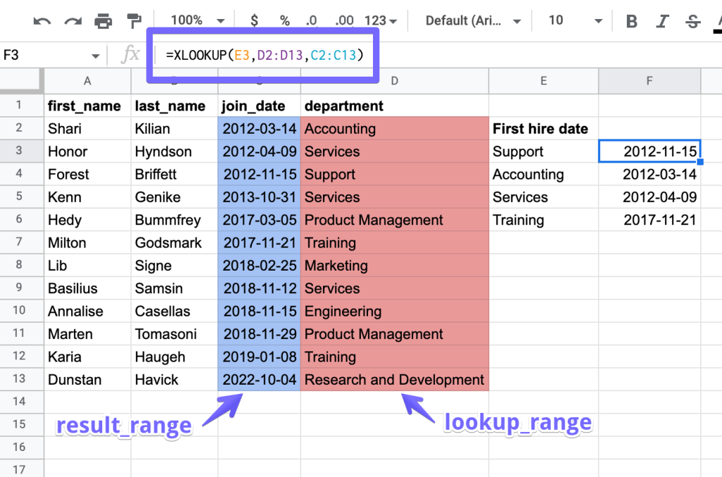
Here, we pick up the value from cell E3, search for it in the ‘department’ column, and return the corresponding date from the ‘join_date’ table. The search works exactly as in VLOOKUP.
XLOOKUP with horizontal lookup
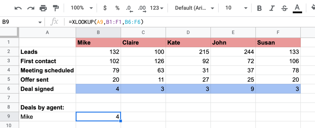
Horizontal lookup in XLOOKUP Google Sheets works in a similar fashion to the vertical one. In the table below, we have the sales pipeline for each of our agents. We use the following formula to pick up the number of signed deals by Mike:
=XLOOKUP(A9,B1:F1,B6:F6)
For that, we scan row 1 in search of ‘Mike’ and for the found cell, we return the value in row 6:
XLOOKUP with multiple columns as a result
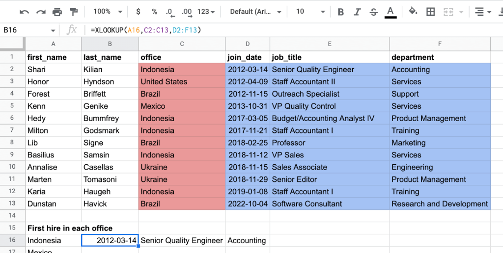
XLOOKUP can return not just one but multiple adjacent cells as a result of a single function. It’s a common use when you, for example, look up information on a certain client or an employee and want to know quite a few things about them.
A Google Sheets XLOOKUP formula could look as follows:
=XLOOKUP(A16,C2:C13,D2:F13)
In our example, we’re scanning the employees’ table to find the details of the first person hired in each office. We search through the ‘office’ column and return the corresponding results from columns ‘join_date’, ‘job_title’, and ‘department’.
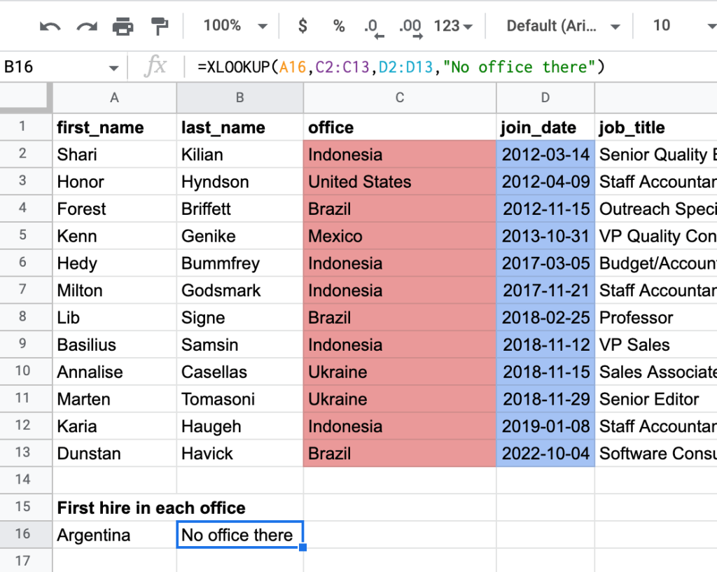
XLOOKUP with missing value
If the search_key doesn’t exist in the lookup_range, you would normally see an error like this:
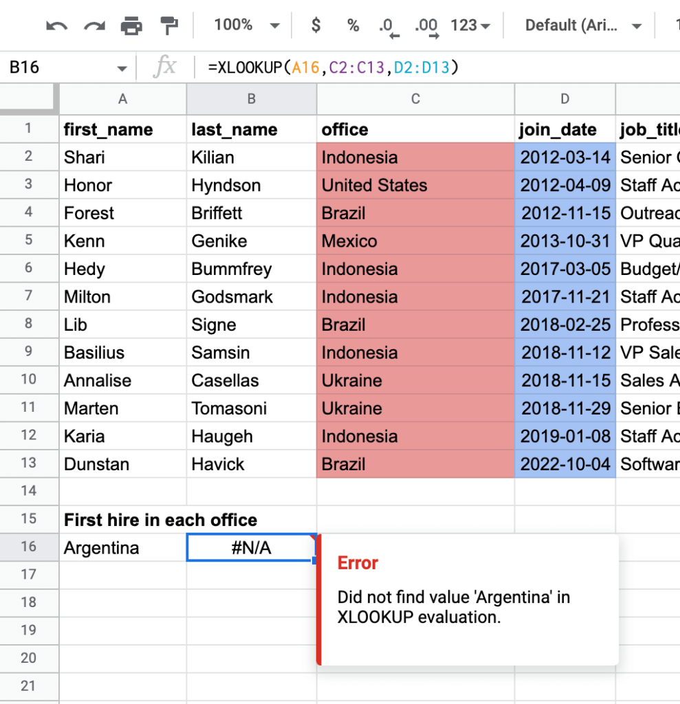
Google Sheets XLOOKUP lets you remove that ugly error and place a customized, more meaningful text there instead.
=XLOOKUP(A16,C2:C13,D2:D13,"No office there")
XLOOKUP with an approximate match
Now, let’s jump to the fifth parameter called [match_mode] where you can choose from four different options. As a reminder:
| Selection | Match mode behavior |
| 0 | Exact match. |
| -1 | Exact match but if no match, the first value lower than the search_key will be returned. |
| 1 | Exact match but if no match, the first value higher than the search_key will be returned. |
| 2 | Partial match with the use of wildcards (?, *, ~). |
The ‘0’ selection (exact match) is the default one and we used it in the previous examples. If no exact match is found, the XLOOKUP function in Google Sheets returns either a #N/A error or a fallback message specified in the [missing_value] parameter.
By choosing ‘-1’ or ‘1’, you can take advantage of an approximate match. XLOOKUP will look precisely for the value you picked as a search_key but if it fails to find one, it will pick the next in order. It will be:
- The first lower value than the
search_keyfor ‘-1’ - The first higher for ‘1’
Let’s look at an example. In the following table, we have the list of employees from our sales teams with their sales last month. Based on these sales, they’re eligible for a bonus that they’ll get upon reaching a certain threshold. For example, sales of $40,000-$49,999 will guarantee a 20% bonus.
To find the bonus value for the first employee, we use the following XLOOKUP Google Sheets formula:
=XLOOKUP(D2,$F$3:$F$7,$G$3:$G$7,,-1)
We pick up their sales number, search for it in the red column, and return the value from the blue column. Before spreading this formula onto the other rows, we freeze the lookup_range and result_range to continue checking the very same cells. Here’s the result:
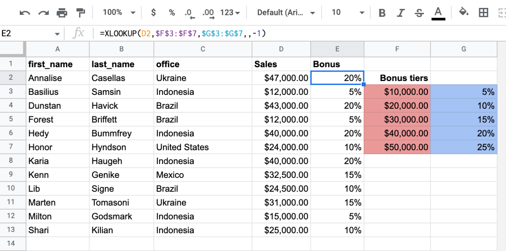
Notice that you can skip the earlier [missing_value] parameter by leaving it blank.
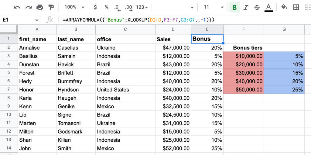
XLOOKUP with an ARRAYFORMULA
The XLOOKUP function above works perfectly on a small dataset but as the list of rows grows, it’s better to use an ARRAYFORMULA instead. The function will populate all rows by default. If you need to add or remove any data, the ARRAYFORMULA will make sure the relevant XLOOKUP formula is in place.
In the E1 cell, we paste the following formula:
=ARRAYFORMULA({"Bonus";XLOOKUP(D2:D,F3:F7,G3:G7,,-1)})
The function places a “Bonus” label in the E1 cell and inserts the relevant formula into each subsequent row. As we add Mr John Smith to the mix (row 14), the bonus is calculated automatically without the need for any adjustments.
XLOOKUP with a wildcard
Google Sheets XLOOKUP supports three wildcards:
- * (asterisk) that represents zero or more characters
- ? (question mark) that matches precisely one character
- ~ (tilde) that nullifies the effect of other wildcards so that you can search for either character
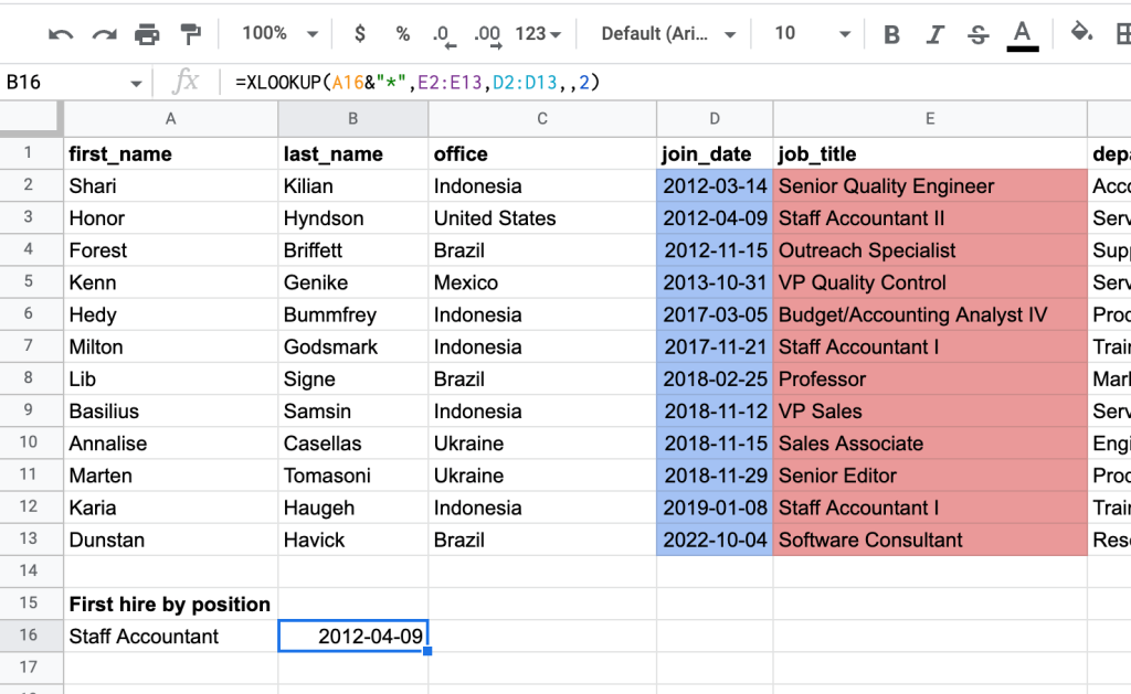
Jumping back to the earlier dataset, we have the list of employees with their job titles. Some positions, for example, Staff Accountant, have different levels to them. In this example, we want to find the start date of the first Staff Accountant on our employees’ list, regardless of the level assigned to their position.
For that, we’ll use the * wildcard and the following formula:
=XLOOKUP(A16&"*",E2:E13,D2:D13,,2)
And here’s the result:
XLOOKUP with the search bottom to top
Now let’s look at the last, optional parameter of the XLOOKUP formula in Google Sheets. As a reminder, the possible selections are as follows:
| Selection | Match mode behavior |
| 1 | Search from the first entry to the last. |
| -1 | Search from the last entry to the first. |
| 2 | Search the lookup_range using the binary search, assuming it’s sorted in ascending order. |
| -2 | Search the lookup_range using the binary search, assuming it’s sorted in descending order. |
By default, the function uses the ‘1’ selection, meaning that it searches from the first entry to the last, exactly the same as VLOOKUP and HLOOKUP do. There can be, however, situations when you want to search from the last entry to the top.
For example, in the function below we want to fetch the sales of the least successful employee in a particular office:
=XLOOKUP(F4,C2:C13,D2:D13,,,-1)
And the result is:
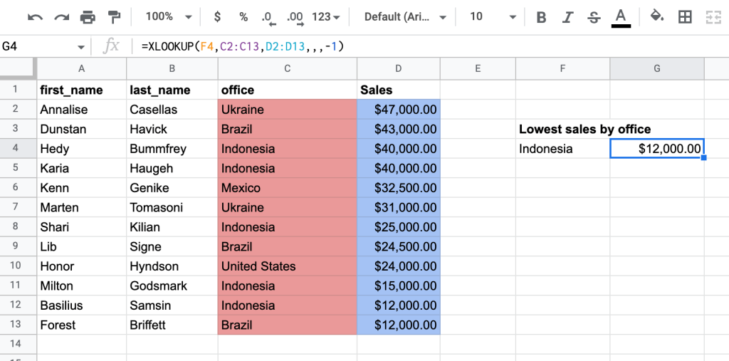
Notice the three commas before the last parameter. In this case, we skipped the previous two parameters and only opted for adjusting the search_mode.
XLOOKUP with the binary search
One more cool thing that XLOOKUP in Google Sheets enables you to use is a binary search. Binary search is extremely useful when processing large datasets that go into thousands or tens of thousands of records as it makes the operations much faster and more efficient.
If you’re unfamiliar with the concept, here’s a simple example. Suppose we have a sorted list of integers from 1 to 7 (1, 2, 3, 4, 5, 6, 7). The search_key in XLOOKUP is 5. The binary search algorithm does the following:
- It compares the search_key against the middle element of the array (4). If they don’t match, the half of the array where the
search_keycan’t exist is discarded. Here, 5 (search_key) > 4 so all elements below 4 are discarded. - It repeats the process on the remaining elements of the array (4, 5, 6, 7). The middle value is 5.5, still different from
search_keyand since 5 < 5.5, integers 6 and 7 are discarded. - 4 and 5 are left. The process repeats again. The middle value is 4.5, 5 > 4.5 so 4 is discarded. The winner is 5!
In this example, XLOOKUP had to perform just three comparisons to get to the desired result and with a bit of luck, it could have stumbled upon ‘5’ even earlier. Using the regular search mode of XLOOKUP, it could take up to seven comparisons to get the desired result. When dealing with thousands of records at the time, it could make a difference.
Now, let’s look at a different example. We have a dataset with the list of employees and there are literally thousands of them. Each has a number of days they have stayed at the company. We sorted the table by this column, descending.
We want to know if someone is celebrating a 500, 1,000, or 3,000 days-at-the-company anniversary. Rather than scroll through the table every time we need such data, we can use the XLOOKUP formula instead.
=XLOOKUP(E3,$C$2:C,$A$2:B,,,-2)
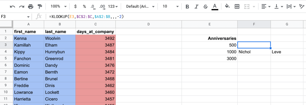
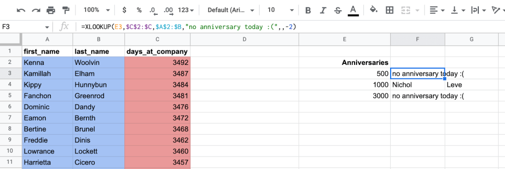
Since we didn’t specify the fifth parameter of the function ([match_mode]), XLOOKUP Google Sheets assumes we’re only interested in an exact match. No one is apparently celebrating a 500-day or 3,000-day anniversary today, so XLOOKUP returns empty cells. It may seem confusing at first, so adding an error message as a fourth parameter would be probably a good idea.
=XLOOKUP(E3,$C$2:$C,$A$2:$B,"no anniversary today :(",,-2)
XLOOKUP in Google Sheets – wrapping up
We hope the examples we’ve shared were useful in understanding the full scope of what’s possible with XLOOKUP Google Sheets. Should you have any questions or face unexpected errors, be sure to check Google’s documentation online.
Lastly, if Google Sheets is the centre of operations for your business, you may find Coupler.io useful for automating your workflows. We use it ourselves to pull data from the various business apps we use and we can’t imagine going back to manual exports. Check if it could work for you too.
Thanks for reading!