Excel is a great tool for storing and managing your data. However, looking through each entry can be overwhelming when it comes to understanding what all that data is telling us. You often want to aggregate or summarize your data to better understand any trends, rankings, or other insights hidden in the data.
Have you heard of Excel’s AGGREGATE function? Well, it’s a powerful tool that allows you to calculate sums, averages, counts, and many other types of data aggregations. It can even ignore error values and hidden rows if needed.
This article will go over the syntax and usage of AGGREGATE, as well as some examples. So, read on to learn about this amazing function! ?
How to aggregate data in Excel
You can aggregate data in Excel using several different methods:
#1: Using aggregate functions
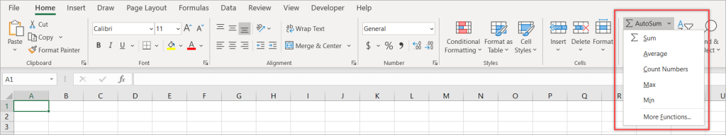
Aggregate functions calculate a set of values and return a single value as a summary result. The five most common functions are SUM, AVERAGE, COUNT, MAX, and MIN—which you may already be familiar with. There’s even an AutoSum button in the Home tab for these functions so that you don’t have to manually type them.
There are also functions such as SUMIF/SUMIFS, COUNTIF/COUNTIFS, MAXIFS, MINIFS, etc., to help you summarize data using specific criteria. Statistical functions such as MODE and MEDIAN are also available.
Additionally, Excel has special functions like AGGREGATE and SUBTOTAL that bring together many aggregate functions into one convenient package.
The AGGREGATE function is the focus of this article. And if you haven’t heard of or used the AGGREGATE function before, don’t worry; we cover that later in this article.
#2: Other options: Pivot tables and Power Query
Both are great for summarizing and analyzing your data.
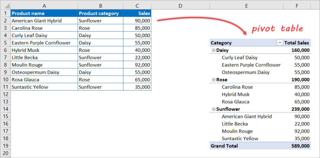
You may want to use Power Query’s data transformation tools to apply groupings or use aggregate functions to summarize your data. Or, you may want to use a pivot table to create a nice table visualization containing aggregated values as shown below:
Before summarizing your data using one of these tools, it’s not uncommon that you need to get raw data from an external source and do some cleanups. With Excel Power Query, you can easily create connections from many external sources, and also use them when creating pivot tables.
Now, what if you need to import data from many different sources, but are not familiar using Power Query?
An alternative is using an integration tool such as Coupler.io that allows you to import data from various sources into Excel without coding! With this tool, you can easily get data from apps such as Jira, QuickBooks, Shopify, Hubspot, and more!

Don’t forget to check out Microsoft Excel integrations supported by Coupler.io.
Now, what is the AGGREGATE function in Excel?
When you’re summarizing data using aggregate functions, a single cell’s error could cause the formulas not to work. There are situations when you just don’t have time to fix errors in your data. Especially, when you’re processing a large amount of data.
Fortunately, there is this function called AGGREGATE that was introduced in Excel 2010. You can use it as a multipurpose function to do different data aggregations like finding sums, averages, etc. while ignoring errors and hidden rows.
AGGREGATE formula in Excel: Syntax and parameters
The Excel AGGREGATE function can have two syntax forms: reference and array syntaxes.
Syntax
Reference form:
=AGGREGATE(function_num, options, ref1, [ref2], ...)Array form:
=AGGREGATE(function_num, options, array, [k])You do not need to worry about which form you are using. Excel will select the appropriate form based on the input parameters you specify.
Parameters or arguments
The following are the parameters used in the AGGREGATE function.
| Parameter | Explanation |
|---|---|
function_num | Required. A number 1 to 19 that specifies which aggregate function is to be performed. |
options | Required. A number 0 to 7 that determines what to ignore in the evaluation range for the function. |
ref1, [ref2], … | ref1: Required. A reference to the range of cells on which the function is to be applied.[ref2], …: Optional. Additional range of cells. There can be up to 253 separate ranges (including ref1), each separated by a comma. |
array, [k] | array: An array of values or an array formula upon which the function is to be applied.[k]: A second argument that is required by certain functions when using an array of values or an array formula.See the following functions that require the [k] argument: LARGE(array, k) — k is the nth largest value to be found.SMALL(array, k) — k is the nth smallest value to be found.PERCENTILE.INC(array, k) — k is the percentage value, must be between 0 and 1.QUARTILE.INC(array, quart) — quart is the quartile, must be 0, 1, 2, 3, 4.PERCENTILE.EXC(array, k) — k is the percentage value, must be between 0 and 1. QUARTILE.EXC(array, quart) — quart is the quartile, must be 0, 1, 2, 3, 4. |
There are 19 different aggregate functions you can use with AGGREGATE. While it doesn’t cover all of the aggregate functions in Excel, it does offer a wide range of choices. You also have 8 choices to specify how hidden cells and errors are handled using this function.
The 19 functions supported by AGGREGATE
The table below lists the aggregate functions you can use with AGGREGATE. The values 1-19 in the first column are used as the first argument of this function.
| function_num | Aggregate function |
|---|---|
| 1 | AVERAGE |
| 2 | COUNT |
| 3 | COUNTA |
| 4 | MAX |
| 5 | MIN |
| 6 | PRODUCT |
| 7 | STDEV.S |
| 8 | STDEV.P |
| 9 | SUM |
| 10 | VAR.S |
| 11 | VAR.P |
| 12 | MEDIAN |
| 13 | MODE.SNGL |
| 14 | LARGE |
| 15 | SMALL |
| 16 | PERCENTILE.INC |
| 17 | QUARTILE.INC |
| 18 | PERCENTILE.EXC |
| 19 | QUARTILE.EXC |
Here are options to specify how errors and hidden rows are handled using AGGREGATE. The values 0-7 in the first column of the table below are used as the second argument of this function.
| options | What to ignore |
|---|---|
| 0 or [blank] | Ignore nested SUBTOTAL and AGGREGATE functions |
| 1 | Ignore hidden rows, nested SUBTOTAL, and AGGREGATE functions |
| 2 | Ignore error values, nested SUBTOTAL, and AGGREGATE functions |
| 3 | Ignore hidden rows, error values, nested SUBTOTAL, and AGGREGATE functions |
| 4 | Ignore nothing |
| 5 | Ignore hidden rows |
| 6 | Ignore error values |
| 7 | Ignore hidden rows and error values |
Please note, the AGGREGATE function is designed to work only with vertical ranges, so there is no option to ignore hidden columns.
You may be wondering what SUBTOTAL is. Well, it’s a function that works similarly to AGGREGATE. However, SUBTOTAL supports only 11 aggregate functions, and there is no option to ignore errors.
How to use AGGREGATE function in Excel: Basic usage
Let’s take a look at how to use this function with a basic example.
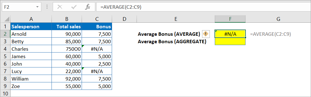
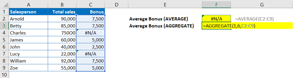
Suppose you have the following data and want to find the average bonus given to salespeople. As you can see, there are cells with #N/A errors in the range C2:C9. If you use the AVERAGE function on this range, you will also get an #N/A result — see the following screenshot:
Now, let’s use AGGREGATE in F3 to find the average by following the steps below:
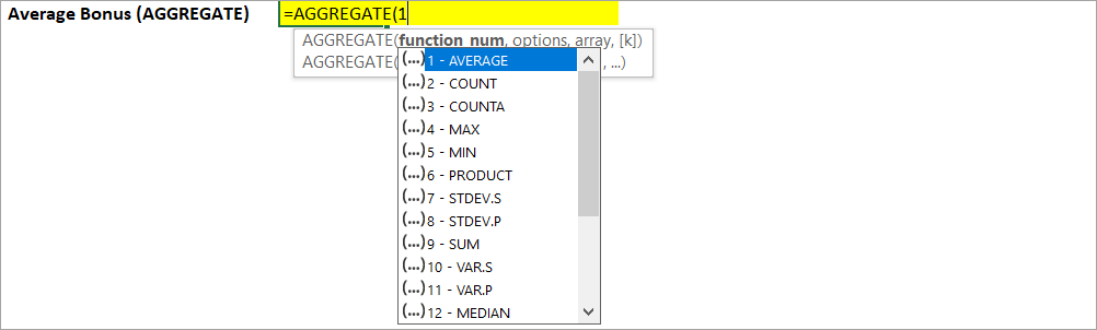
Step 1: Type =AGGREGATE(. You will see a list of aggregate functions appear in a dropdown.
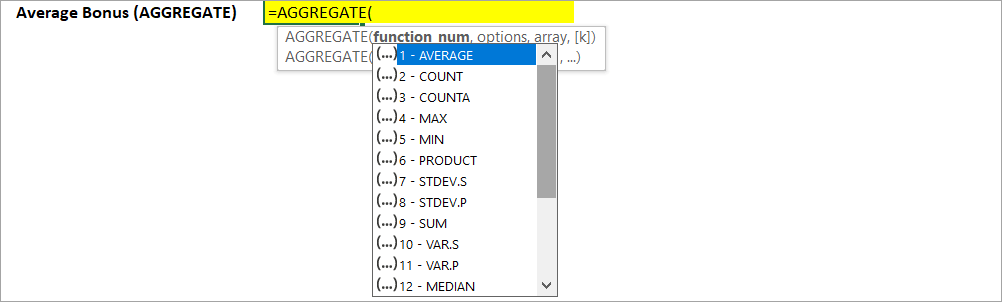
Step 2: Manually type the function number (function_num) you want to use, or just double-click it. In this case, enter 1, which is the number for the AVERAGE function.
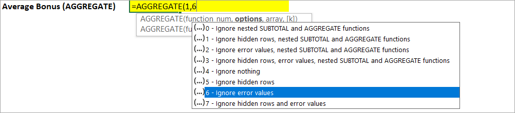
Step 3: Type a comma, and in the options list that appears, select 6 to ignore errors.
Step 4: Type a comma again. After that, enter the range you want to calculate and close the bracket.
Step 5: Press Enter.
Here’s the AGGREGATE Excel formula we use in F3:
=AGGREGATE(9,6,D2:D11)
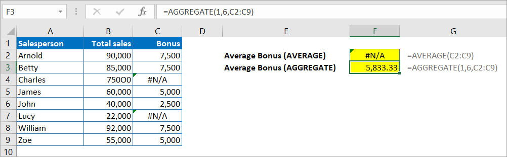
The function returns an average result (function_num = 1) of the values in the range C2:C9. It allows us to ignore any errors in the range and returns a result. As you can see, the result of this function is not an #N/A error like the result of the AVERAGE function in F2.
Excel AGGREGATE function: More examples
Let’s see more examples of how to use AGGREGATE in different scenarios.
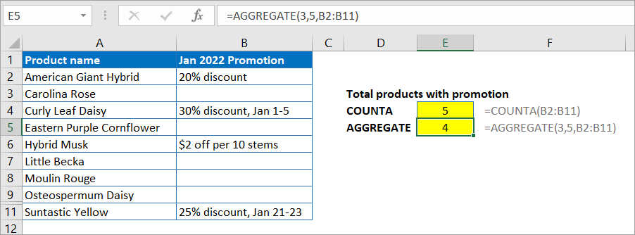
With the following data, suppose you want to know how many products are in January 2022 promotions. To do that, you calculate the number of cells in B2:B11 that are not blank using the COUNTA function in E4.
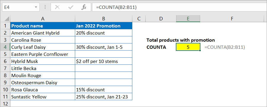
With Rosa Glauca set to be discontinued in January 2022, you might want to hide Row 10 manually. However, when printing the data with summary info, this could cause confusion. That’s because the COUNTA’s result will be the same even after the row is hidden.
One way around this problem is using AGGREGATE with COUNTA function to ignore hidden rows, as follows:
=AGGREGATE(5,3,D2:D11)
Example #2: Aggregation Excel – multiple references
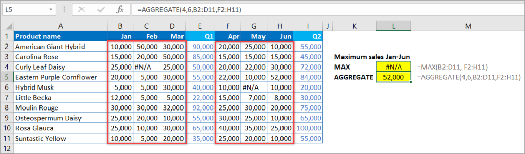
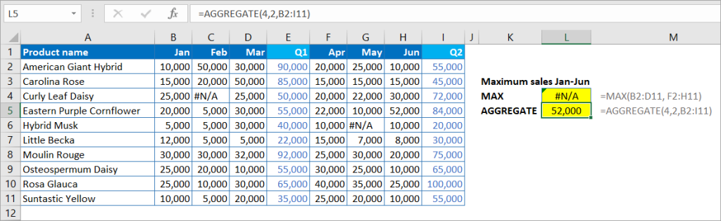
In the following example, we calculate the maximum amount of sales in January – June, which are in ranges B2:D11 and F2:H11. Notice that the MAX function in L4 returns an error, while AGGREGATE doesn’t.
Here’s the AGGREGATE formula we use in L5 that uses MAX (function_num = 4) while ignoring errors (options = 6).
=AGGREGATE(4,6,B2:D11,F2:H11)
Example #3. Aggregation Excel – Ignore nested AGGREGATE
For this example, we’ll use the same case and data as Example #2 above. We are going to calculate the maximum amount of sales in January – June. But now, we are using range B2:I11 instead of multiple references.
Let’s take a closer look at the calculations in columns Q1 and Q2 that use AGGREGATE with SUM by ignoring error values, as shown in the following screenshot:
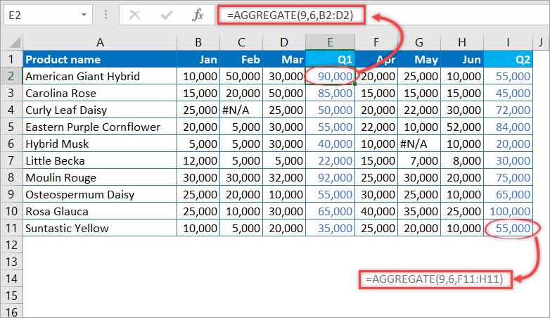
To find the maximum values in January – June, we can simply use this AGGREGATE formula that ignores errors and nested AGGREGATE (options = 2):
=AGGREGATE(4,2,B2:I11)
Example #4. Excel AGGREGATE function with [k] parameter
Suppose you have the following product sales data and want to calculate the 1st, 2nd, and 3rd largest sales:
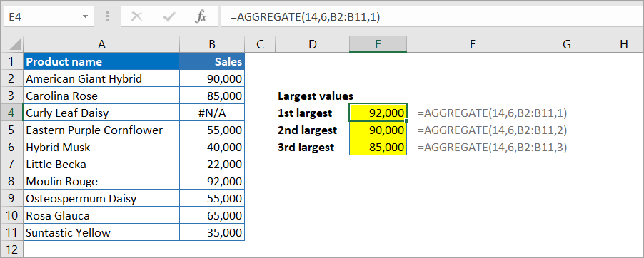
As shown in the above screenshot, here are the formulas in E4, E5, and E6:
=AGGREGATE(14,6,B2:B11,1)
=AGGREGATE(14,6,B2:B11,2)
=AGGREGATE(14,6,B2:B11,3)
The AGGREGATE formulas above use LARGE (function_num = 14) in range B2:B11 while ignoring errors (options = 6).
Notice that the [k] parameter is the nth largest value to be found in the range. Please note that if you don’t provide a value for this parameter, AGGREGATE returns a #VALUE! error.
Example #5. Excel AGGREGATE function with [k] parameter and array formula
Let’s see a more complex example that uses an array formula.
The following AGGREGATE formulas are used to calculate the 1st, 2nd, and 3rd smallest values of product sales for products in the “Sunflower” category.
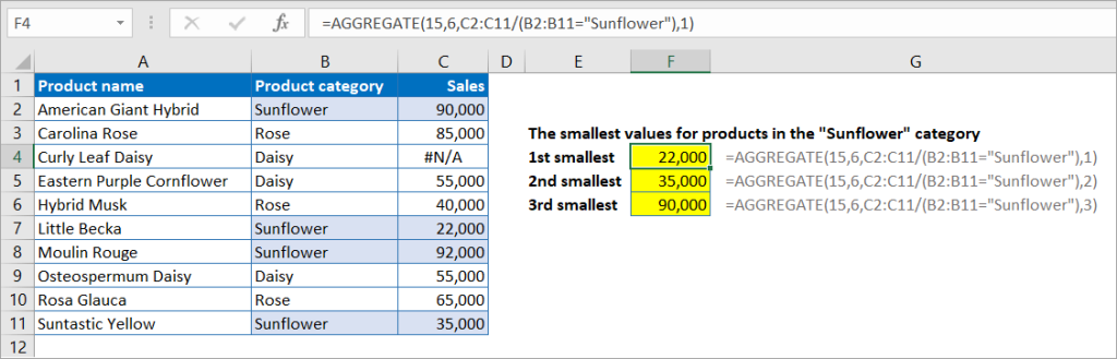
The formulas in E4, E5, and E6 are:
=AGGREGATE(15,6,C2:C11/(B2:B11="Sunflower"),1)
=AGGREGATE(15,6,C2:C11/(B2:B11="Sunflower"),2)
=AGGREGATE(15,6,C2:C11/(B2:B11="Sunflower"),3)
Notice that the AGGREGATE formulas above use SMALL (function_num = 15) in range C2:C11 where values in B2:B11 equal “Sunflowers”. All errors are ignored (options = 6).
Here’s how Excel evaluates the formula to find the smallest value:
- The logical expression
B2:B11="Sunflower"returns an array of TRUE/FALSE values:{TRUE;FALSE;FALSE;FALSE;FALSE;TRUE;TRUE;FALSE;FALSE;TRUE}. - The
C2:C11/(B2:B11="Sunflower")evaluates to:{90000;85000;#N/A;55000;40000;22000;92000;55000;65000;35000} /({TRUE;FALSE;FALSE;FALSE;FALSE;TRUE;TRUE;FALSE;FALSE;TRUE}). - FALSE evaluates as zero and throws a #DIV/0! error. TRUE evaluates as 1 and returns the original value. Thus, the previous expression becomes:
{90000;#DIV/0!;#N/A;#DIV/0!;#DIV/0!;22000;92000;#DIV/0;#!DIV/0!;35000}. - The final formula:
=AGGREGATE(15,6,{90000;#DIV/0!;#N/A;#DIV/0!;#DIV/0!;22000;92000;#DIV/0;#!DIV/0!;35000},1)returns 22000, which is the smallest value in the array.
Isn’t it interesting that you don’t need to press Ctrl+Shift+Enter when using AGGREGATE with an array formula? ?
What is table aggregation in Excel?
Well, it’s simply an aggregation applied to an Excel table. You’ll find it easier and more flexible than doing it on ranges of data.
So, when you have data in rows and columns in Excel, formatting it as a table will give you more benefits. For example, filtering or aggregating your data becomes easier and more time-saving.
If you don’t know how to format your data as a table, follow the steps below:
Click on any cell of your data, then click the Insert tab on the ribbon and click Table. Then, in the “Create Table” dialog that appears, click OK if the data range and header option are correct.
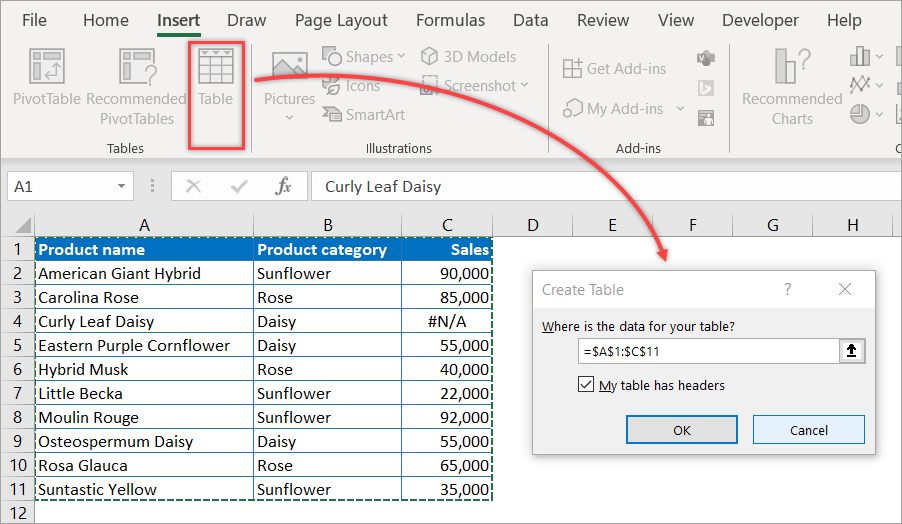
After that, Excel creates a table for you.
In the Table Design tab, you can see the default name of your table. You can rename it, as well as change other settings such as table formatting and style.
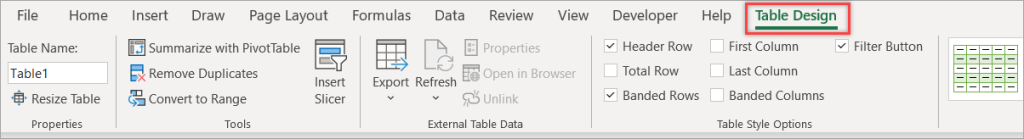
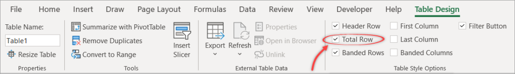
To apply aggregation to your table, you can easily tick the Total Row option in the Table Style Options group:
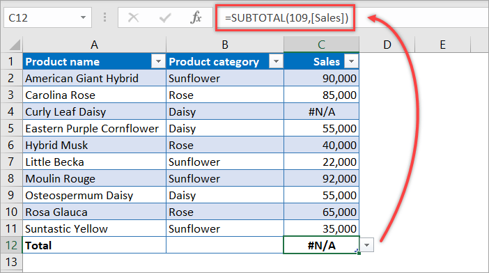
You will see a summary row added at the bottom, and by default, it uses a SUBTOTAL function, which allows you to include or ignore hidden rows but not error values:
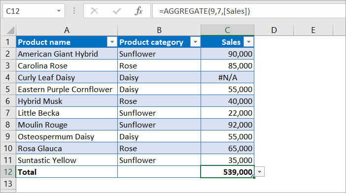
However, you can change it to use other functions such as SUM, AVERAGE, AGGREGATE, etc., by using the dropdown in the Total row or writing your own.
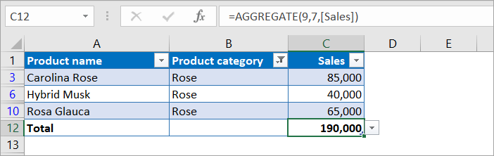
For example, here we use an AGGREGATE function to sum the Sales (function_num = 9) by ignoring errors and hidden rows (options = 7). We get the following result, which is not an #N/A error:
=AGGREGATE(9,7,[Sales])
Now, if you filter the table, you’ll see that the total is automatically updated to ignore hidden rows:
Should you change an aggregation function in Excel to use AGGREGATE?
You’ve seen how the AGGREGATE function in Excel can be so powerful because it supports 19 aggregate functions and can ignore errors, hidden rows, and nested AGGREGATE or SUBTOTAL.
That makes AGGREGATE perfect for replacing those 19 aggregate functions!
So, should you use it all the time?
Well, if you want, of course you can! There are many good reasons to use AGGREGATE. This function can do 152 different things (19 functions x 8 options), handle array formulas for certain functions, and is very fast to use on a large dataset.
However, please keep in mind that this function is only available in Excel 2010 or later versions. It’s also more complicated to use it than using SUM, COUNT, or other aggregate functions.
So, in some cases, you may want to simply use aggregate functions instead of AGGREGATE. For example, when your dataset is not too large, and you have time to correct any errors in your data.
Finally, thanks for reading—and happy summarizing!
