Sometimes analyzing a huge set of data can be a pain. This is why important tools like BigQuery have been developed and are constantly evolving. With Google BigQuery, you can simplify your analytics processes, analyze your data with ease, and extract critical insights using simple SQL and many of its predefined functions.
This article covers one of the most potent yet complex sets of functions: Window Functions. Understanding how to effectively use BigQuery Window Functions will power up your analytics capabilities and help you extract all the important information out of your data.
What are BigQuery Window Functions
BigQuery Window Functions, also known as Analytic Functions, is a set of functions that helps you compute values over a group of rows and return a single result for each row.
This is extremely useful in situations where you need to calculate important metrics such as moving averages and cumulative sums, and perform other types of analyses over your data. Below is a brief table with all the different functions that can be used for window calculations:
| Function Name | Function Description |
|---|---|
| Aggregation Functions | |
ANY_VALUE | Returns the value of a random row in a selected group. |
ARRAY_AGG | Returns an array with the values of the selected group. |
AVG | Returns the average of non-NULL values in a group. |
CORR | Returns the Pearson coefficient of correlation between the given pair. The first number is used as the dependent variable, while the second number is the independent variable. |
COUNT | Returns the number of rows in the input. |
COUNTIF | Returns the number of rows in the input where the expression provided is evaluated to TRUE. |
COVAR_POP | Returns the population covariance of a set of number pairs. |
COVAR_SAMP | Returns the sample covariance of a set of number pairs. |
MAX | Returns the maximum value of non-NULL expressions. |
MIN | Returns the minimum value of non-NULL expressions. |
ST_CLUSTERDBSCAN | This can be used on a column of geographies and performs a DBSCAN clustering returning the zero based cluster number. |
STDDEV_POP | Returns the population standard deviation of the given values. |
STDDEV_SAMP | Returns the sample standard deviation of the given values. |
STRING_AGG | Returns a STRING value that is the concatenation of the given non-NULL values. |
SUM | Returns the sum of non-NULL values. |
VAR_POP | Returns the population variance of the given values. |
VAR_SAMP | Returns the sample variance of the given values. |
| Navigation Functions | |
FIRST_VALUE | Returns the value of the first row in the current window frame. |
LAST_VALUE | Returns the value of the last row in the current window frame. |
NTH_VALUE | Returns the value of the nth row in the current window frame. |
LEAD | Given an offset, returns the value of a subsequent row in the current window frame. |
LAG | Given an offset, returns the value of a preceding row in the current window frame. |
PERCENTILE_CONT | Computes the specified percentile value for a set of values, with linear interpolation. |
PERCENTILE_DISC | Computes the specified percentile value for a set of discrete values. |
| Numbering Function | |
RANK | Returns the ordinal rank of each row within the ordered partition. |
DENSE_RANK | Returns the ordinal rank of each row within each window partition. |
PERCENT_RANK | Returns the percentile rank of a row in a specific partition. |
CUME_DIST | Returns the relative rank of a row in a specific partition. |
NTILE | This function divides the rows into constant_integer_expression buckets based on row ordering and returns the bucket number that is assigned to each row. |
ROW_NUMBER | Returns the sequential row ordinal for each row. |
BigQuery Window Function vs. Aggregate Functions
As you may have noticed, the above looks a lot like simple aggregate functions like summing a set of rows or calculating their average. BigQuery Window Functions are similar, with the only difference being that they are used to calculate and return a result for each row instead of a single result for the whole set. In standard aggregate functions, the resulting data are grouped by a set of dimensions, while in window functions, we can preserve our rows and show each result along them.
A BigQuery Window Function example
Enough with the theory; let’s go and see what a BigQuery Window Function looks like. First, let’s see how we can construct a BigQuery Window Function syntax-wise:
bigquery_window_function_name ([argument_list])
OVER (
   [PARTITION BY window_partition]
   [ORDER BY order_expression { ASC | DESC } ]
   [{ROWS | RANGE} frame_clause]
)
The above syntax follows the below notation rules:
- Square brackets “
[ ]” indicate optional clauses. - Parentheses “
( )” indicate literal parentheses. - The vertical bar “
|” indicates a logical OR. - Curly braces “
{ }” enclose a set of options.
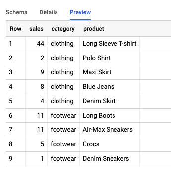
To see a BigQuery Window Function in action, we need to load an example set of data into BigQuery. Our table “Sales” for this example comes from a JSON file that looks like below:
{'product': 'Long Sleeve T-shirt', 'category': 'clothing', 'sales': 44}
{'product': 'Long Boots', 'category': 'footwear', 'sales': 11}
{'product': 'Polo Shirt', 'category': 'clothing', 'sales': 2}
{'product': 'Maxi Skirt', 'category': 'clothing', 'sales': 9}
{'product': 'Blue Jeans', 'category': 'clothing', 'sales': 8}
{'product': 'Air-Max Sneakers', 'category': 'footwear', 'sales': 11}
{'product': 'Crocs', 'category': 'footwear', 'sales': 5}
{'product': 'Denim Skirt', 'category': 'clothing', 'sales': 4}
{'product': 'Denim Sneakers', 'category': 'footwear', 'sales': 1}
If you already have your dataset in BigQuery, that’s great; you are ready to run the examples. If not, Coupler.io allows you to automate the load of your data from a wide range of sources to BigQuery using one of many BigQuery integrations.
To do this, sign up to Coupler.io for free and complete three steps:
- Set up your data source
- Set up BigQuery as the data destination
- Set up your schedule
You can also load data from JSON APIs without any coding using the dedicated JSON to BigQuery integration.
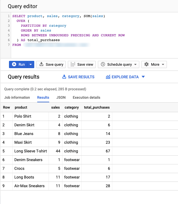
Below is an example of calculating the cumulative sum of purchases per category using Window Functions:
SELECT product, sales, category, SUM(sales)
  OVER (
    PARTITION BY category
    ORDER BY sales
    ROWS BETWEEN UNBOUNDED PRECEDING AND CURRENT ROW
  ) AS total_purchases
FROM Sales
Don’t worry if the above query doesn’t make any sense. We will go through many examples below, and by the end of this article, you will be able to use BigQuery Window Functions in your own queries.
BigQuery Window Functions: Use OVER in Standard SQL
First of all, let’s see what the OVER clause means in a query and how you can define it. The OVER clause references a window that defines a group of rows in a table. Upon this window, you can use an analytic function and calculate your required metric.
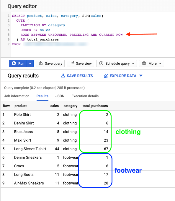
Let’s see in depth the example we used above and try to understand how OVER is used:
SELECT product, sales, category, SUM(sales)
  OVER (
    PARTITION BY category
    ORDER BY sales
    ROWS BETWEEN UNBOUNDED PRECEDING AND CURRENT ROW
  ) AS total_purchases
FROM Sales
Using this query, our plan is to calculate the cumulative sum of sales for each category while mapping each sale next to it. So to do that, first, we SELECT our result columns (product, sales, category, SUM(sales)).
Following that, we have to define over which group of rows these results will be calculated using the OVER clause. We first PARTITION BY category in order to define which column will be used to group our rows and calculate the SUM of the sales, which in this case, is the category column.
Then, we order the set by sales and specify the upper and lower boundaries of our set using the ROWS BETWEEN UNBOUNDED PRECEDING AND CURRENT ROW command. This command sets the frame’s lower bound to infinite, and the upper bound is the current row each time, so the query will calculate the SUM from the start of the set until each respective row, ending up with the below result:
How to use BigQuery Window Functions between dates
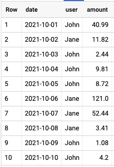
Many of the cases where Window Functions are used are to calculate rolling metrics between dates. Let’s see an example where we have a table that logs the transactions of different users across time and looks like below:
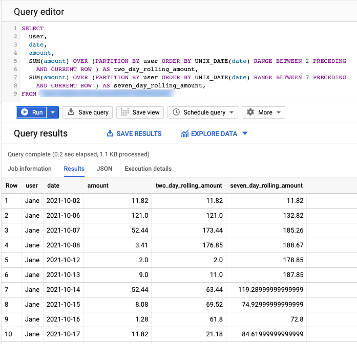
Let’s say we want to calculate the total amount for each user in 2-day and 7-day sliding windows. To do that, we can use the below query:
SELECT user, date, amount, SUM(amount)
  OVER (
  PARTITION BY user
  ORDER BY UNIX_DATE(date)
  RANGE BETWEEN 2 PRECEDING AND CURRENT ROW
  ) AS two_day_rolling_amount,
  SUM(amount)
  OVER (
  PARTITION BY user
  ORDER BY UNIX_DATE(date)
  RANGE BETWEEN 7 PRECEDING AND CURRENT ROW
  ) AS seven_day_rolling_amount,
FROM Sales;
We used two different SUM calculations wherein the OVER clause we ordered by date and used two different windows to calculate between specific days (2 days preceding current row and until current row):
RANGE BETWEEN 2 PRECEDING AND CURRENT ROWRANGE BETWEEN 7 PRECEDING AND CURRENT ROW
With these windows, we can calculate the cumulative sum looking back 2 and 7 days accordingly. The results of the above query will look like below:
BigQuery Window Functions: What is LAG and how to use it
Navigation functions are a subset of Window Functions and are frequently used to access a specific set of rows. LAG is maybe one of the most popular and widely used navigation functions.
LAG returns the value expression on a preceding row defined by a specific offset. Let’s see a specific example applied to the query we used above:
SELECT
  user,
  date,
  amount,
  LAG(amount, 2) OVER (PARTITION BY user ORDER BY UNIX_DATE(date)) AS two_day_rolling_amount,
  LAG(amount, 7) OVER (PARTITION BY user ORDER BY UNIX_DATE(date)) seven_day_rolling_amount,
FROM Sales
Using LAG we can access the amount spent exactly 2 or 7 days prior to the specific row date. Running this query will return the below table. Please note that when the offset is NULL or a negative value, the returned value is always NULL.
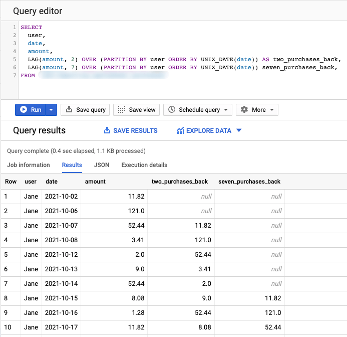
For reference, you can use other navigation functions in a similar manner:
FIRST_VALUELAST_VALUENTH_VALUELEADLAGPERCENTILE_CONTPERCENTILE_DISC
How to skip NULL values in BigQuery Window Functions
When navigation functions are used, there are times where NULL values need to be ignored. For example, if you’re looking for the first and second available preceded value, you might want to ignore the NULLS.
To do that, we can use the IGNORE NULLS value expression as shown below:
SELECT
  runner,
  finish,
  division,
  tag,
  NTH_VALUE(tag, 1 IGNORE NULLS) OVER (PARTITION BY division ORDER BY finish DESC ROWS BETWEEN 1 FOLLOWING and UNBOUNDED FOLLOWING) AS previous_tag1,
  NTH_VALUE(tag, 2 IGNORE NULLS) OVER (PARTITION BY division ORDER BY finish DESC ROWS BETWEEN 1 FOLLOWING and UNBOUNDED FOLLOWING) AS previous_tag2
FROM Runners
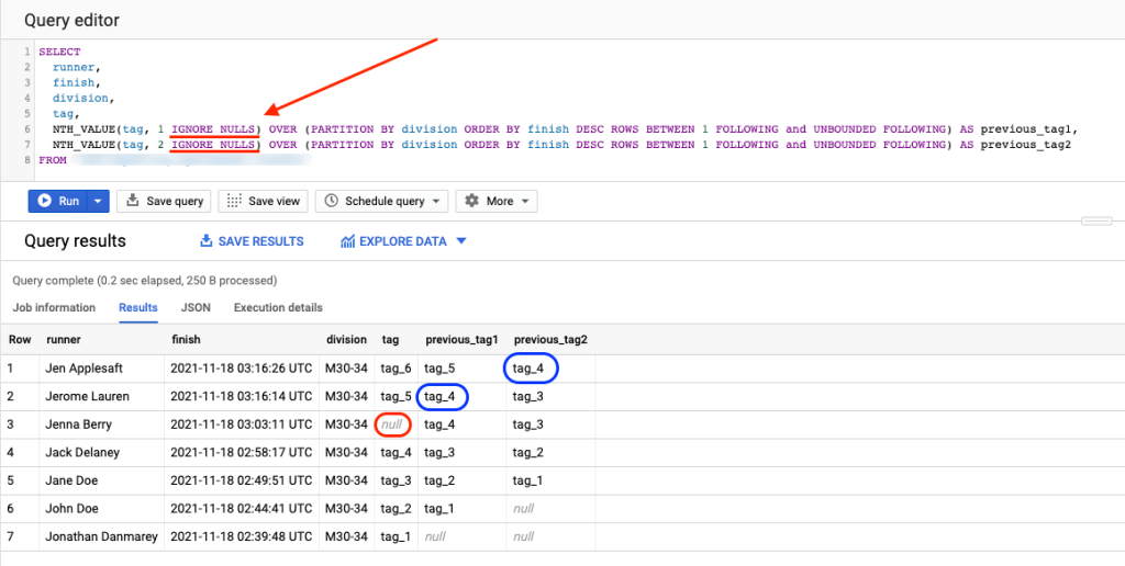
As you can see, even though the tag record in row 3 is NULL, previous_tag1 and previous_tag2 in rows 2 and 1, respectively (blue highlight) show a value, and they ignored the NULL tag (red highlight).
BigQuery Window Functions: What is RANK and how to use it
Now it’s time to go over another popular function used in Window Functions: RANK. It returns the ordinal (1-based) rank of each particular row in the order partition provided. All peer rows receive the same rank value. The next row or set of peer rows receives a rank value which increments by the number of peers with the previous rank value.
This is extremely useful as ranking is one of the most popular actions. For example, let’s say we have a dataset with runners in a marathon, and we want to rank them and find each one’s position. The initial table looks as below:
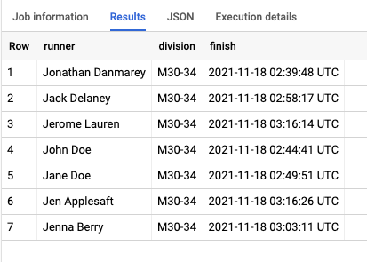
To rank them in order and calculate their position, we can use the below query:
SELECT
  runner,
  division,
  finish,
  RANK() OVER (PARTITION BY division ORDER BY finish) AS position
FROM
  Runners
Which will rank all the runners as shown below:
BigQuery Window Functions: Use filters
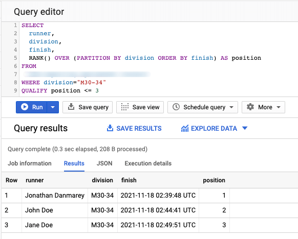
There are many cases where you might want to filter the results of a Window Function. This can be done by using the QUALIFY clause. QUALIFY filters the results of Window Functions, and only rows that are evaluated as TRUE will be included.
Let’s see QUALIFY in action using the above example of runners. If we want to filter in and keep only the runners that made the podium (top 3) in a specific division, we can use QUALIFY as shown below:
SELECT
  runner,
  division,
  finish,
  RANK() OVER (PARTITION BY division ORDER BY finish) AS position
FROM
 Runners
WHERE division="M30-34"
QUALIFY position <= 3
How to calculate standard deviation
Last but not least, let’s see how we can calculate standard deviation by taking advantage of BigQuery Window Functions. Currently, two statistical aggregate functions can calculate Standard Deviation:
STDDEV_POPSTDDEV_SAMP
STDDEV_POP returns the population (biased) standard deviation of the values, while STDDEV_SAMP returns the sample (unbiased) standard deviation of the values.
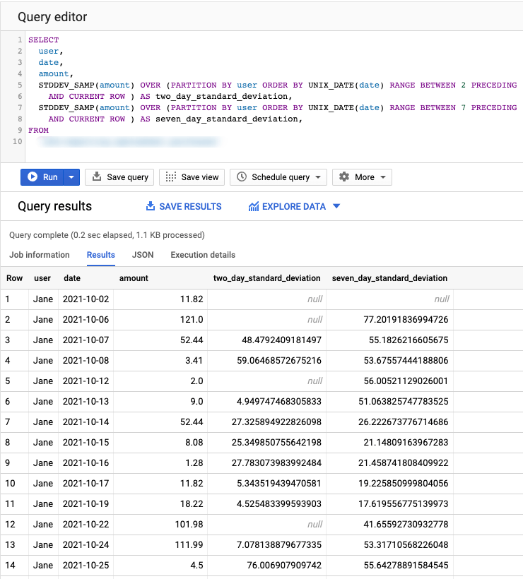
Both of these functions can be used along with Window Functions and take advantage of the OVER clause to calculate their values over a specified window. Let’s use STDDEV_SAMP on our Sales table below to calculate standard deviation over a 2-day and 7-day window:
SELECT
  user,
  date,
  amount,
  STDDEV_SAMP(amount) OVER (PARTITION BY user ORDER BY UNIX_DATE(date) RANGE BETWEEN 2 PRECEDING
    AND CURRENT ROW ) AS two_day_standard_deviation,
  STDDEV_SAMP(amount) OVER (PARTITION BY user ORDER BY UNIX_DATE(date) RANGE BETWEEN 7 PRECEDING
    AND CURRENT ROW ) AS seven_day_standard_deviation,
FROM
  Sales
Wrapping up
This article has gone through all the important aspects of BigQuery Window Functions, from the initial theory to specific examples. Of course, BigQuery Window Functions cannot be learned in a night, but we think reading this article will give you a solid initial foundation to build upon.
Like everything, you can only get good with practice, and Window Functions are worth the effort as they can be really useful on your analytics projects. So, don’t waste any more time; load your data in BigQuery (if you haven’t already) and try to see how BigQuery Window Functions work in action!
