Excel SUMIF with Text Criteria: Formula Examples

In most cases in your day-to-day data analysis, you probably just want a quick way to sum cells based on text criteria. For example, if you have a list of product sales and want to calculate the total sales by product type, or maybe to sum based on products with names containing specific text. Excel’s SUMIF function is a powerful and simple way to add up values based on criteria. In this article, you’ll learn how to use this function with text-based criteria in different situations. 

How to use SUMIF with text criteria in Excel

SUMIF allows you to sum numbers based on criteria. To use SUMIF with text criteria, you can use the following general formula:

=SUMIF(criteria_range, "text_criteria", [sum_range])

Where:

• criteria_range: The range of cells that contains the criteria.
• "text_criteria": Text criteria, enclosed in double quotes.
• [sum_range]: The range of cells to add. This parameter is optional. If you don’t specify this argument, Excel adds the cells specified in the criteria_range argument.

Here are some important notes:

• The text criteria is not case-sensitive. 
• The length of the text criteria is limited to 255 characters.
• You can use logical operators (=, >, >=, <, <=, <>) combined with text criteria. However, you can omit the “=” operator when using “is equal to” criteria. 
• You can use the text criteria with wildcards (*, ?, ~) for partial matching.
• If you want to find the sum of values with multiple criteria, use the SUMIFS function instead.

Also, keep in mind that you can also use SUMIF with dates or numbers in the criteria other than text. If you want to learn about the basics of SUMIF, check out our article on that: SUMIF function in Excel.

Basic Examples of Excel SUMIF function with text criteria

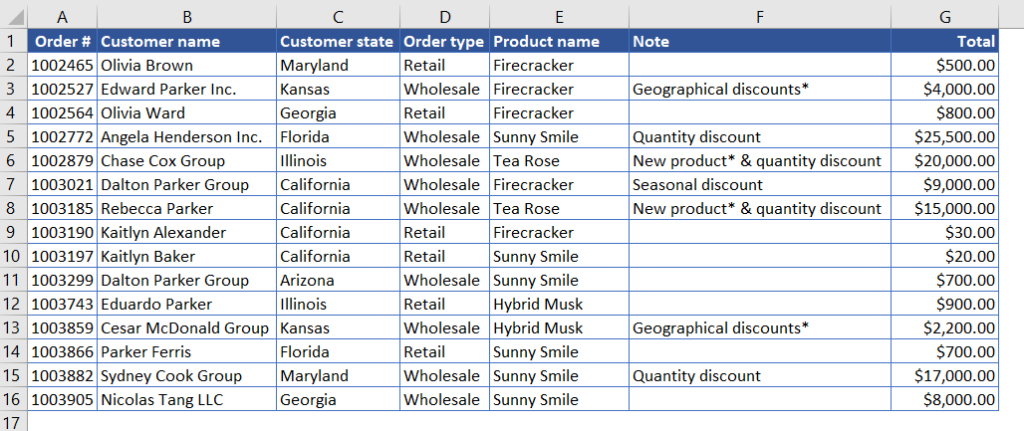
We’ll use the following order data for most of the examples used in this article. As you can see, each order has an order number, order type, customer info and the product they ordered, total order value in USD, and notes related to that particular order. 

Tip: If you have data stored in PipeDrive, Shopify, Jira, or other external sources but want to do an analysis using Excel, you can import them first into Excel using Coupler.io. It’s a powerful data integration tool that lets you bring data from external sources into Excel, Google Sheets, and BigQuery for your analysis needs! Explore Microsoft Excel integration, as well as how Coupler.io works and reasons you would need Excel integration for your business.

Now, let’s see some examples of using the Excel SUMIF function to solve simple cases, such as summing if cells match specific text, if cells are empty, etc. 

Excel SUMIF: If cells match specific text

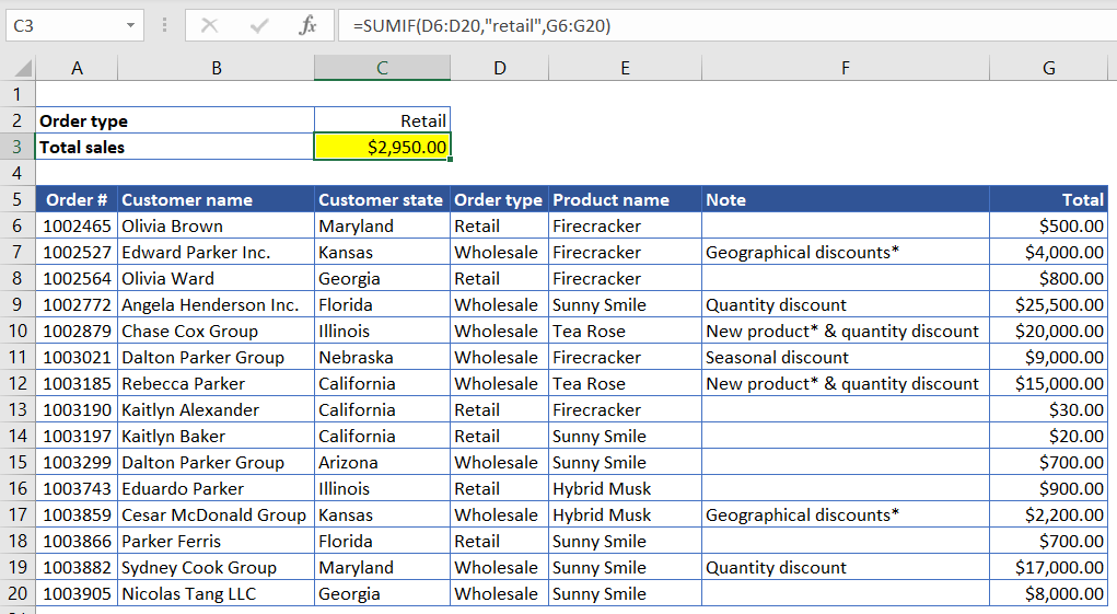
In the following example, we are calculating the total for Retail orders using a SUMIF formula in C3:

Formula explanation:

=SUMIF(D6:D20,"retail",G6:G20)

The formula sums the amounts in column G (range G6:G20), where the order type in column D (D6:D20) is equal to "retail". Notice that the text is enclosed within double quotes and not case-sensitive. You can also write it as either "RETAIL" or "Retail", and the total will be the same.

You can also refer to C2 instead of typing the text criteria manually. To do that, just replace “retail” with C2 (without double quotes): 

=SUMIF(D6:D20,C2,G6:G20)

Excel SUMIF: If cell does not equal text

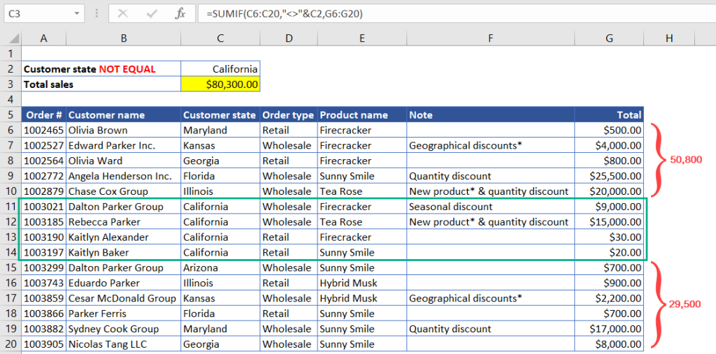
In the following example, we calculate the total order by non-California customers.

Formula explanation:

=SUMIF(C6:C20,"<>"&C2,G6:G20)

The formula calculates the total orders in range G6:G20, where the customer’s state in range C6:C20 does not equal California. Notice that in the criteria parameter, we use the "<>" operator combined with cell C2, which refers to "California".

Excel SUMIF: If text is empty, not empty (blank, not blank)

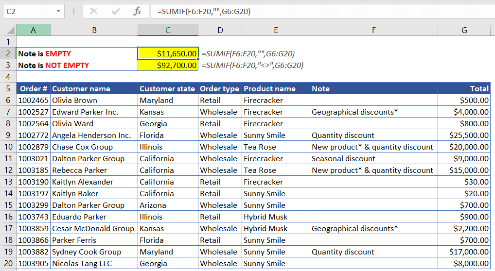
As you can see in the following screenshot, some orders have notes while others don’t. In this example, we are comparing the total sales for orders with empty notes vs. not empty.

Formula explanation:

We use the following formulas in C2 and C3:

• Note is empty (C2): =SUMIF(F6:F20,"",G6:G20)
• Note is not empty (C3): =SUMIF(F6:F20,"<>",G6:G20)

Notice that we use "" (double quotes, without any space between them) to find empty notes. To search for anything that is not empty, we use "<>" (not equal operator, wrapped in double-quotes).

Examples of Excel SUMIF with criteria: cell contains partial text

SUMIF supports using wildcards for partial matching, which makes this function powerful. You can use the following wildcard characters to perform partial searches:

Use	To find
? (question mark)	Any single character. For example, ?ike finds "Bike" and "Nike".
* (asterisk)	Any sequence of characters. For example, Ja* finds "Jane" and "Jake".
~ (tilde) followed by ?, *, or ~	A question mark, asterisk, or tilde.  A tilde in front of a wildcard character is an escape character for that wildcard.  For example, Bob~? finds "Bob?".

Now, let’s see some examples below for using SUMIF with wildcards.

Excel SUMIF: If cell contains specific text in any position

Suppose we want to calculate the total sales generated by customers with a name containing “Parker”, and then put the result in C2, as the following screenshot shows:

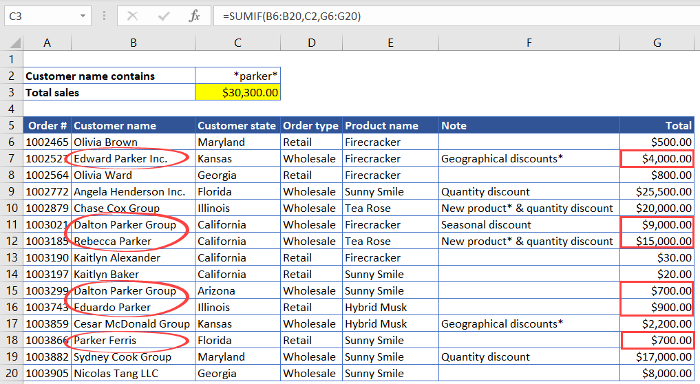
Formula explanation:

=SUMIF(B6:B20,C2,G6:G20)

The SUMIF formula in C3 has the text criteria *parker*. If you notice, it finds the rows with the customer name containing “parker” in any position: start, middle, or end. If we entered the text criteria directly in the formula, we would need to enclose it with double-quotes, and the formula would look like this:

=SUMIF(B6:B20,"*parker*",G6:G20)

Notice again that the criteria is not case-sensitive.

Excel SUMIF: If cell starts or ends with specific text

In the following example, we will calculate the total orders for customers whose name starts with "Olivia" in C2 and customers whose name ends with "Group" in C3.

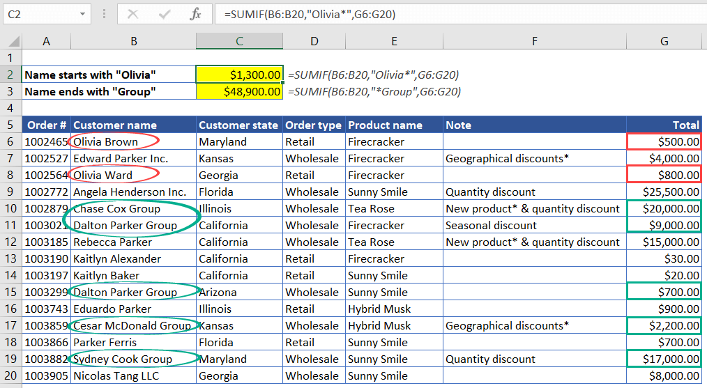
Formula explanation:

We use the following formulas in C2 and C3:

• Name starts with “Olivia” (C2): =SUMIF(B6:B20,"Olivia*",G6:G20)
• Name ends with “Group” (C3): =SUMIF(B6:B20,"*Group",G6:G20)

To search for all text starting with "Olivia", we add an asterisk at the end of the criteria: "Olivia*". To match all text ending in "Group", we place an asterisk at the beginning of the criteria: "*Group".

Excel SUMIF: If cells contain an asterisk 

The following example shows how to calculate the total for orders with a note containing an asterisk (*) in C2; whereas in C3, the formula calculates the total for orders with a note containing an asterisk at the end.

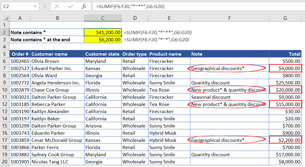
Formula explanation:

• Note contains * (C2): =SUMIF(F6:F20,"*~**",G6:G20)
• Note contains * at the end (C3): =SUMIF(F6:F20,"*~*",G6:G20)

The asterisk itself is a wildcard that represents any number of characters. So, if you want to find text with an asterisk in it, use a tilde (~) before the asterisk character, to indicate the character itself (and not a wildcard). 

More advanced examples of Excel SUMIF with text criteria

We’ll see some examples of using SUMIF in Excel with multiple text criteria. In addition, we’ll see how to sum based on color using VBA.

Excel SUMIF with multiple “OR” text criteria

With the following table, suppose we want to add up the total orders made by customers from Arizona or Illinois.

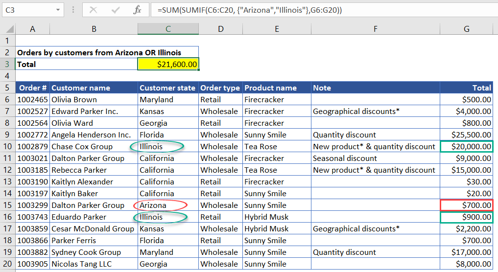
Formula explanation:

=SUM(SUMIF(C6:C20, {"Arizona","Illinois"},G6:G20))

Notice that in the criteria, we use an array with two text elements: {"Arizona","Illinois"}. The SUMIF function can take an array in its criteria argument. But this will force the function to also return the results as an array: {700,20900}, which is the total orders for Arizona and Illinois, separately. This is why it’s necessary to wrap the SUMIF within SUM. The SUM does the final work by adding up each element in the array and returning 21600, which is the correct result.

Excel SUMIFS with multiple “AND” text criteria

In the following example, let’s say we want to calculate the total Wholesale orders by customers from Kansas.

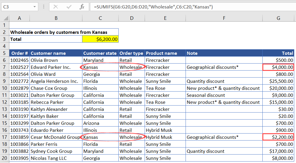
Formula explanation:

=SUMIFS(G6:G20,D6:D20,"Wholesale",C6:C20,"Kansas")

In this case, we use the SUMIFS function instead of SUMIF in the formula because SUMIFS supports multiple criteria. Notice that we place the range that we want to sum in the first parameter when using this function, followed by each pair of criteria range and criteria.

Excel SUMIF based on text background color

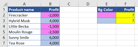
With the following table, suppose we want to calculate the total profit based on the cell background color. 

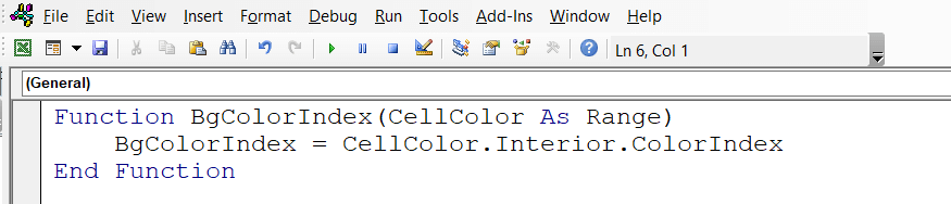
There is no default function in Excel to find the total based on a cell’s background color. One of the solutions is to create a VBA function to get the color index of the background color and use it with SUMIF. Here’s how:

1. Press Alt+F11 to open the Visual Basic Editor (VBE).
2. Click Insert > Module.
3. Copy-paste the following function to the editor:

Function BgColorIndex(CellColor As Range)
    BgColorIndex = CellColor.Interior.ColorIndex
End Function

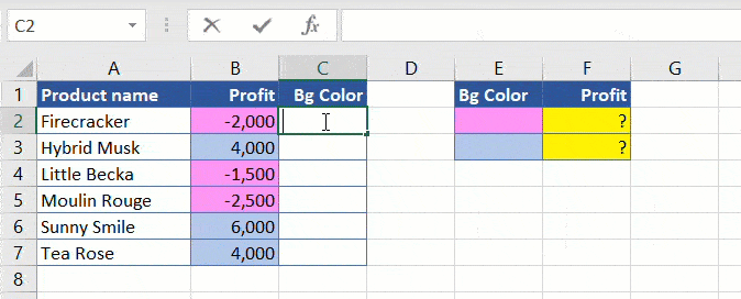
4. Set the header of column C as “Bg Color”. Then, enter =BgColorIndex(B2) in cell C2 and copy it down to row 7.

5. In E2 and E3, write the results returned by the BgColorIndex function for each background color.

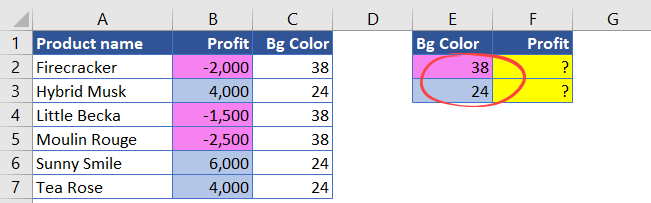
6. Use the following formulas to sum the total based on the criteria in E2 and E3:
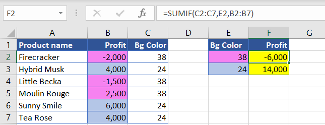
   1. Color index is 38 (cell F2): =SUMIF(C2:C7,E2,B2:B7)
   2. Color index is 24 (cell F3): =SUMIF(C2:C7,E3,B2:B7)

You will get the following result:

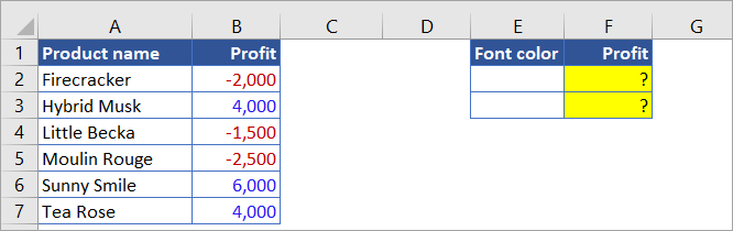
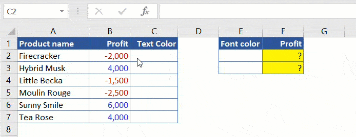
Excel SUMIF based on text color

Now, what if we want to sum based on text color (font color)? The solution is similar to our previous example, but instead of getting the index of the background color, we’re getting the index of the text color. After that, we’ll use SUMIF to sum the total. 

Here are the steps:

1. Press Alt+F11 to open the Visual Basic Editor (VBE).
2. Click Insert > Module.
3. Copy-paste the following function to the editor:

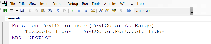
Function TextColorIndex(TextColor As Range)
    TextColorIndex = TextColor.Font.ColorIndex
End Function

4. Set the header of column C as “Text Color”. Then, enter =TextColorIndex(B2) in cell C2 and copy it down to row 7. 

5. In E2 and E3, write the results returned by the TextColorIndex function for each text color.

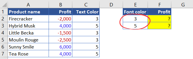
6. Use the following formulas to sum the total based on the criteria in E2 and E3:
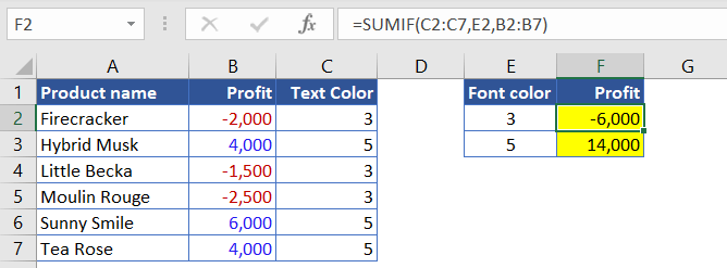
   1. Color index is 3 (F2): =SUMIF(C2:C7,E2,B2:B7)
   2. Color index is 5 (F3): =SUMIF(C2:C7,E3,B2:B7)

You will get the following result:

Wrapping up

We’ve covered various SUMIF formulas for summarizing values ​​based on text criteria in Excel, from basic to more complex scenarios. We hope these examples have been helpful and come in handy when you need to do a quick analysis of your day-to-day work. If you are looking to import data into Excel, BigQuery, or Google Sheets, don’t forget to try Coupler.io. This amazing tool can import data from external sources into Excel, making it easier to analyze — no coding required!

Back to Blog