All you need to know about the Excel SUMIF function, and How to Use it + Examples

Adding up all the numbers in a single column or row in Excel is easy — the SUM function will work just fine. But what if you only want to sum cells that meet a certain condition – for example, to calculate the total sales generated by a specific product? In this case, Excel has a useful function called SUMIF to help you with the job!

Now, let’s go over what the SUMIF function is and how to use it with various examples, so you can see just how helpful this tool can be! 

What is the SUMIF function in Excel?

The SUMIF function is a perfect choice when you’re looking for an easy way to aggregate certain data quickly. Unlike pivot tables, which may require more advanced knowledge in order to use correctly, SUMIF is relatively easy to get started with. 

Here we have a spreadsheet that shows how much revenue was generated by each product and its packaging:

• 

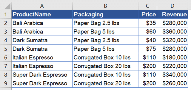
As you’re looking at the above data, the following questions might cross your mind:

• What is the total revenue generated by Bali Arabica?
• What is the total revenue generated from products with prices under $50?
• What is the total revenue generated from products packaged in paper bags?

The SUMIF function can help you answer those questions quickly. With it, you can sum values based on a single criteria, like those specified by the above questions.

Can I use SUMIF with multiple criteria?

SUMIF does not support multiple criteria. For example, you can’t use it to answer questions like: “What is the total revenue generated by products with paper bag packaging AND prices under $50?“. To work around this limitation, you’ll need to use the SUMIFS function, which is the more advanced version of SUMIF. 

So, while SUMIF in Excel is powerful and easy to use, it does have its limitations. For that reason, you will find several examples in this article using SUMIFS as well as other functions as a workaround for solving cases that cannot be solved using SUMIF.

Excel SUMIF syntax and parameters

Syntax

=SUMIF(critera_range, criteria, [sum_range])

Parameters or arguments

Parameters	Description
criteria_range	Required. The range of cells that contains the criteria.
criteria	Required. The criteria used to determine which cells to add. It can be in the form of a number, expression, cell reference, text, or function.  Note: You need to use double quotation marks around any text criteria that include logical or mathematical symbols. If the criteria are numeric, you don’t need double quotes. You can also use logical operators as well as wildcards for partial matching, which makes the function powerful. Logical operators: – Equal to (=)  – Not equal to (<>) – Greater than (>) – Greater than or equal to (>=) – Less than (<) – Less than or equal to (<=) Wildcards: – A question mark (?) — matches any single character.  For example, “T?m” matches “Tim” and “Tom“. – An asterisk (*) — matches any sequence of characters. For example, “*ne” matches “Wayne” and “Jane“. – A tilde (~) followed by ?, *, or ~ — matches a question mark, asterisk, or tilde symbol. For example, “fun~?” matches “fun?“
[sum_range]	Optional. The range of cells to add. If you don’t specify this argument, Excel adds the cells that are specified in the criteria_range argument.

How to use SUMIF in Excel: Basic usage

To have a good understanding of how to use the SUMIF function in Excel, let’s take a look at an example below. Suppose you want to find the total revenue generated by Bali Arabica, and want to store the result in G3.  

• 

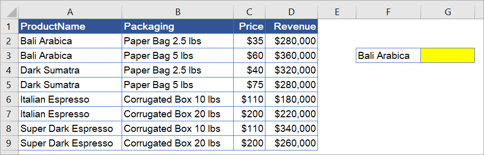
To do that, follow the steps below:

Step 1: Position your cursor on G3 and start entering the formula.

=SUMIF(

Step 2: Enter the range of cells that contains the criteria, which is A2:A9.

=SUMIF(A2:A9

Step 3: Set your criteria in the second argument by typing "Bali Arabica".

=SUMIF(A2:A9,"Bali Arabica"

Note: You can type "bali arabica" or "BALI ARABICA" because SUMIF is not case-sensitive. You can also add the “=” operator in the criteria ("=Bali Arabica"), but the equal sign (=) is not necessarily required when creating the “is equal to” criteria. 

Step 4: Select a range of cells that you want to sum, which is D2:D9. After that, close the parentheses and press Enter.

=SUMIF(A2:A9,"Bali Arabica", D2:D9)

• 

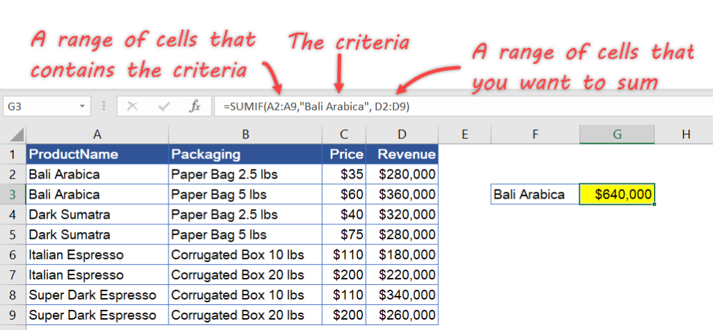
Let’s see what exactly happened:

• Excel searched for the word “Bali Arabica” in the range A2:A9
• If any row had that word, Excel added the revenue value in column D of the same row.
• In the end, you get the sum of all revenue for Bali Arabica.

Note: If your spreadsheet has many rows, using this formula that refers to the entire column may be more convenient:

=SUMIF(A:A,"Bali Arabica",D:D)

Now, if you’d like, try to calculate the revenue generated from Dark Sumatra, Italian Espresso, and Super Dark Espresso. You can follow the same steps as above (Step 1-4).

SUMIF from the Excel ribbon menu

Alternatively, you can insert the SUMIF formula from the ribbon menu. To do that, click Formula, and then in the Function Library section, click Math & Trig. Look for the SUMIF function in the list and select it. 

• 

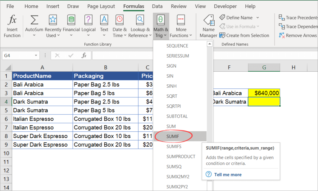
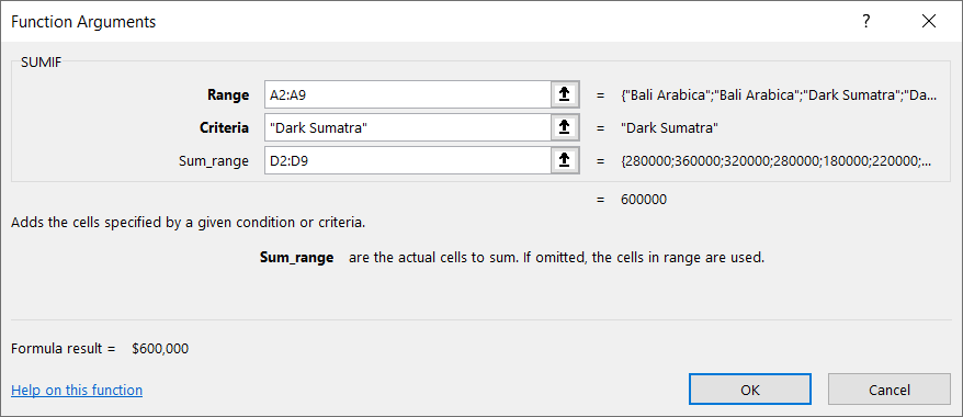
A popup will appear, allowing you to enter the function arguments. See the following arguments for Dark Sumatra. When done, click the OK button.

• 

Excel SUMIF vs. SUMIFS 

When talking about SUMIF, we really must also discuss SUMIFS. Both functions allow you to sum data based on certain conditions. The difference? SUMIF only supports a single criteria, whereas SUMIFS can handle multiple criteria.

SUMIFS syntax

=SUMIFS(sum_range, criteria_range1, criteria1, [criteria_range2, criteria2], …)

The syntax is different from SUMIF in that you need to include the sum_range argument before any other arguments. Also, sum_range is a required argument, not optional like in the SUMIF function. Following the sum_range argument is the pair of the first criteria range and criteria (criteria_range1 and criteria1), and this pair of parameters is also required. 

You can use SUMIFS even for one criteria (like SUMIF). You can add as many criteria as necessary, up to the limit of 127 pairs. 

The basics of how to use these parameters are the same as SUMIF, so we won’t repeat the same explanation here. That means you won’t have to read a longer 😉

How to use SUMIF in Excel if your data is from different sources

Have you ever wanted to analyze data using Microsoft Excel, but your data is stored in external sources such as Jira, PipeDrive, Shopify, etc.? If yes, but you just couldn’t figure out how, our integration tool, Coupler.io, can help you. With this tool, you can import and combine data from different sources into Excel without coding. You can even automate the process on a schedule! 

It’s important to note that your destination file needs to be an Excel Online file on OneDrive. If you want to use a file shared by another user, ensure you have edit access to the file.

To start using Coupler.io, sign up to it (it’s easy and no credit card is required). Then, all you need to do is create a new importer. A wizard will help you configure these three details:

• Source — You can take data from Airtable, Xero, Slack, Trello, and more.

• 

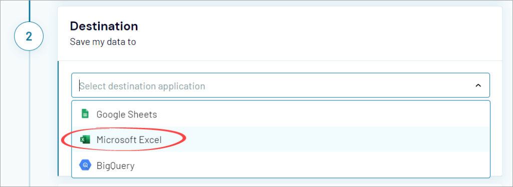
2. Destination — Select Microsoft Excel. 

• 

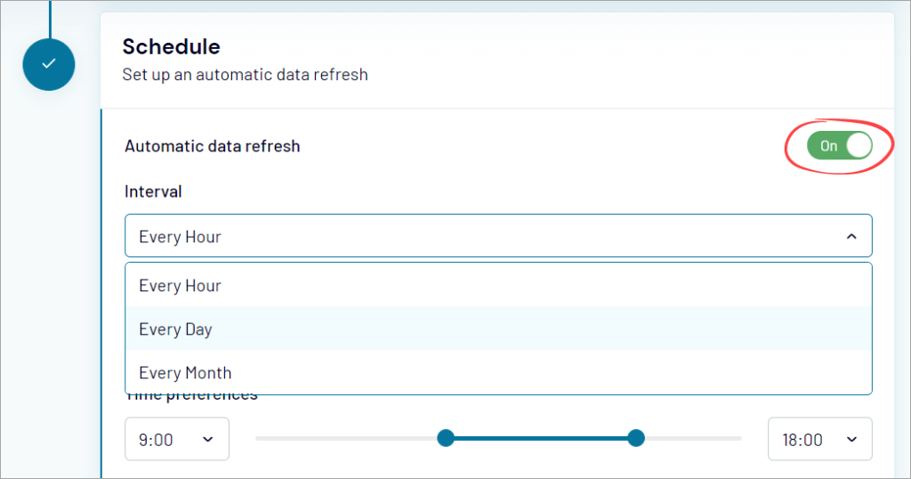
3. Schedule— If you’d like, you can set up automatic data refresh on a schedule: hourly, daily, or monthly.

• 

Pretty easy, right?! Once you finish setting up the importer and run it, your Excel file will be updated. Check out the available Excel integrations.

After that, you can start analyzing your data using Excel. 🙂

Common examples of how to use the SUMIF function in Excel

Understanding the basic use of SUMIF is one thing. But it’s better to be aware that there are many different ways to use this function. Now, let’s look at some common examples so we can get an idea of ​​other fun things we can do with this function.

#1: Excel SUMIF if cells are equal to a value in another cell

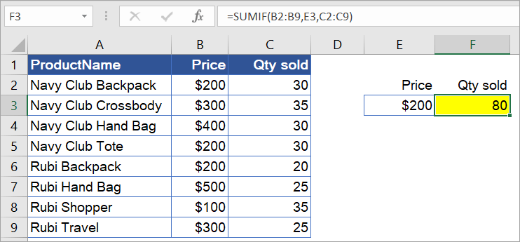
With the data below, suppose you want to find out how many items were sold at $200. You can use this formula:

=SUMIF(B2:B9,200,C2:C9)

But instead of typing 200 manually as the second parameter, you can just refer to E3, as shown in the following formula:

=SUMIF(B2:B9,E3,C2:C9)

• 

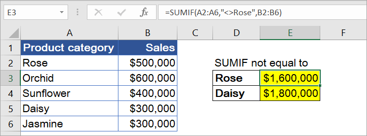
#2: If cells are not equal to

To calculate using the “not equal to” criteria, use the “<>” operator (with double quotes). 

Now, assume that you want to calculate the total sales generated by products other than Rose in E3 and other than Daisy in E4. Use the following formulas:

• Not equal to Rose (E4):

=SUMIF(A2:A6,"<>Rose",B2:B6)

• Not equal to Daisy (E5):

=SUMIF(A2:A6,"<>"&D4,B2:B6)

Notice that for Daisy, we use a cell reference in the formula.

• 

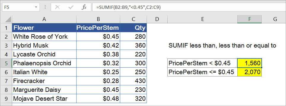
#3: If cells are less than / less than or equal to a number

Use the “<” operator to mean “less than” and “<=” to mean “less than or equal to“. The following example calculates the quantities of flowers with prices per stem that are:

• Less than $0.45 (F5):

=SUMIF(B2:B9,"<0.45",C2:C9)

• Less than or equal to $0.45 (F6):

=SUMIF(B2:B9,"<=0.45",C2:C9)

• 

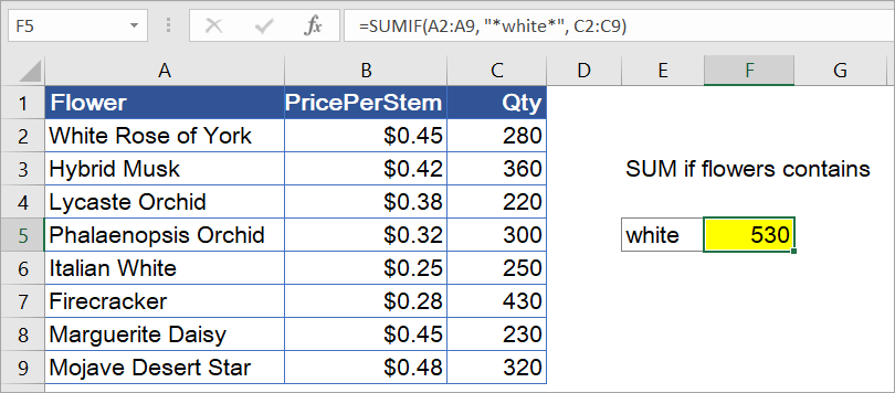
#4: If cell contains text

To sum if cells contain a specific text, you need to use a wildcard when specifying the criteria in the SUMIF function. 

The following example calculates the total quantities of flowers with names containing “white“. Notice again that SUMIF is not case-sensitive. The formula in F5:

=SUMIF(A2:A9,"*white*",C2:C9)

• 

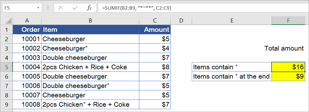
#5: Excel SUMIF if cells contain an asterisk

Asterisks themselves are wildcards. So, to find text that contains an asterisk, you’ll need to use a tilde (~) to treat the character literally (not as a wildcard). The following example shows how to sum the amount for items that:

• Contain * (F5):

=SUMIF(B2:B9, "*~**", C2:C9)

• Contain * at the end (F6):

=SUMIF(B2:B9,"*~*",C2:C9)

• 

#6: Excel SUMIF to sum values based on cells that are blank

Use double quotes without any space in between ("") in the criteria if you want to sum based on cells that are blank. Blank means empty or zero character length.

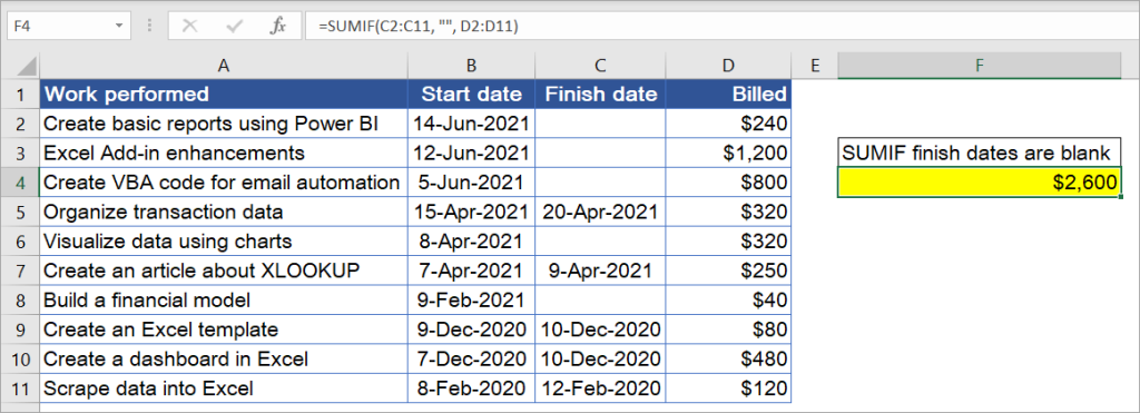
For the following spreadsheet, suppose you want to calculate the total bill for works that are still ongoing (not finished yet). To do that, you calculate the sum based on the finish dates that are blank using the following formula:

=SUMIF(C2:C11,"", D2:D11)

• 

#7: Excel SUMIF to sum values based on cells that are not blank

Use the “not equal to” operator enclosed with double quotes (“<>“) in the criteria if you want to sum based on cells that are not blank.

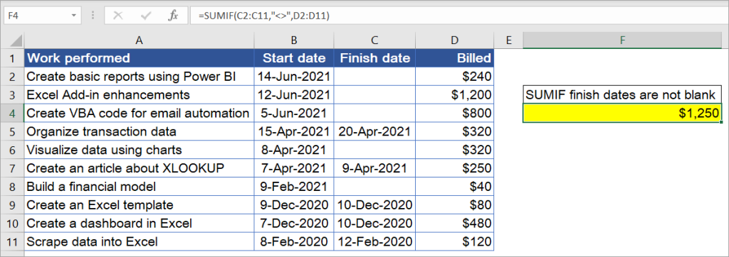
Now, suppose you want to calculate the total bill only for works that are done (finish dates are not empty), use the following formula:

=SUMIF(C2:C11,"<>",D2:D11)

• 

#8: If date is greater than, greater than or equal to

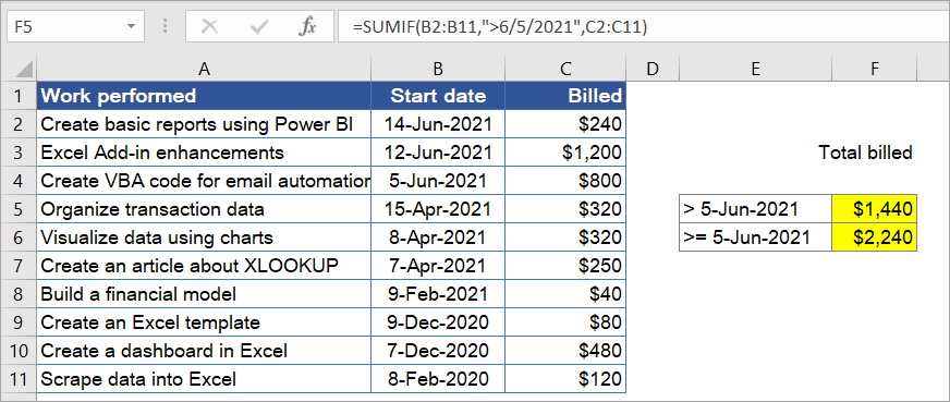
Use the “>” operator for greater than and “>=” for greater than or equal to. The following example sums the total bill for works that started:

• After Jun 5, 2021 (F5):

=SUMIF(B2:B11,">6/5/2021",C2:C11)

• On or after Jun 5, 2021 (F6):

=SUMIF(B2:B11,">="&DATE(2021,6,5),C2:C11)

Notice the formula in F6. You can also use the DATE function in the criteria.

• 

Check out our guide dedicated to Excel SUMIF with Date Criteria.

#9: Excel SUMIF to sum values with the time format

Excel time values are actually numbers and you can sum them up using the SUMIF function like other numeric values. All you need to do is ensure that your data is in the correct time format. But how to set the correct time format? Well, it’s easy. Here’s an example:

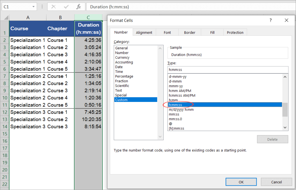
Suppose you want to format Duration (column C) so that it uses the “h:mm:ss” format as shown in the following screenshot:

• 

Follow the simple steps below:

Step 1: Select the entire column C (or only C2:C14 if you want to select this range only).

Step 2: Right-click and select Format Cells. 

Step 3: Click Custom in the category list, then select h:mm:ss on the right. 

Step 4: Click OK.

Now, let’s say you want to sum the total duration for Specialization 2. You can use the following formula:

=SUMIF(A2:A14,E4,C2:C14)

• 

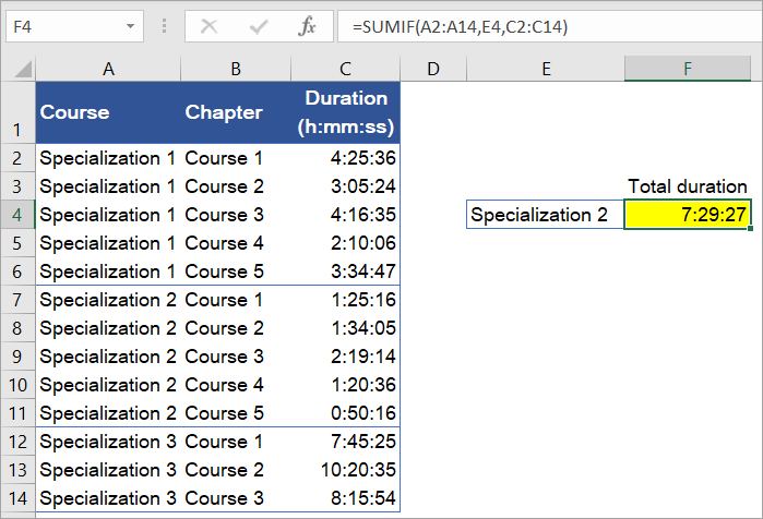
Note: When the sum of time can be greater than 24 hours, you should format the result cells to [h]:mm:ss to avoid the wrong total hours displayed in the results. That’s because for the normal time format like “h:mm:ss”, hours will reset to zero every 24 hours.

#10: With multiple OR criteria

To sum numbers based on other cells being equal to either one value or another, one of the solutions is by using multiple SUMIF functions in one formula.

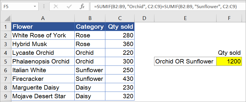
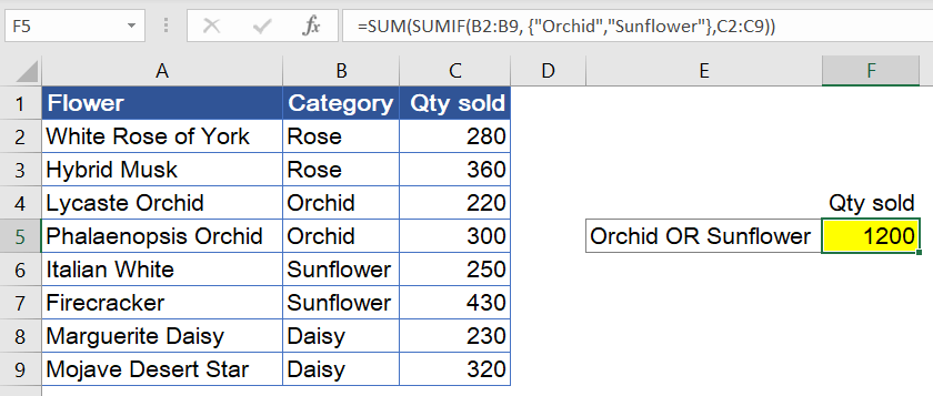
With the following table, suppose you want to sum the quantity sold for either Orchid OR Sunflower. To do that, you can use the following formula:

=SUMIF(B2:B9,"Orchid",C2:C9)+SUMIF(B2:B9,"Sunflower",C2:C9)

• 

The solution here is very simple, and when there are only a few criteria, it often gets the job done quickly. However, if you want to sum values with more than three OR conditions (let’s say), then the formula will become long and complex. To avoid this problem, check out example #11 below, which uses a more advanced method that does not require adding up all of those different parts separately in order to get your total value.

Advanced examples of how to use the SUMIF function in Excel + without Excel SUMIF

Here are some more examples you may find helpful when summing values with criteria.

#11: Excel SUMIF with an array as the criteria argument

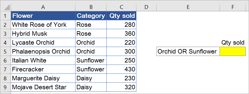
With the following data, suppose you want to sum the quantity sold for either Orchid OR Sunflower. 

• 

Notice that it uses multiple OR criteria, like in example #10. But this time, we’ll use an array in the criteria by following the steps below:

Step 1: List each condition separated by a comma and then enclose with curly brackets: {"Orchid","Sunflower"}

Step 2: Write the complete SUMIF formula using the array:

=SUMIF(B2:B9, {"Orchid","Sunflower"},C2:C9)

• 

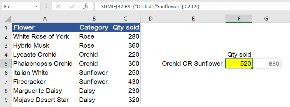
However, when you look at the result, the value is not correct. It only sums the total for Orchid, which is 520. And you’ll also see 680 next to it, which is the total for Sunflower. Why?  

The SUMIF formula takes on an array argument that consists of two values. This forces the formula to return two results separately: 520 and 680. Since we put the formula in cell F5, the function only returns one result for this cell — i.e.,  the total for Orchid.

For this technique to work, you have to use one more step:

Step 3: Wrap your SUMIF formula in a SUM function, as follows:

=SUM(SUMIF(B2:B9, {"Orchid","Sunflower"},C2:C9))

• 

As you can see, the array criteria make the formula much more compact compared to multiple SUMIFs, as seen in example #10. You can also use arrays with numbers, but you don’t need to double-quote them.

#12: With date range criteria (between two dates)

Unfortunately, the SUMIF Excel formula does not work for this case. Instead, you have to use SUMIFS. 

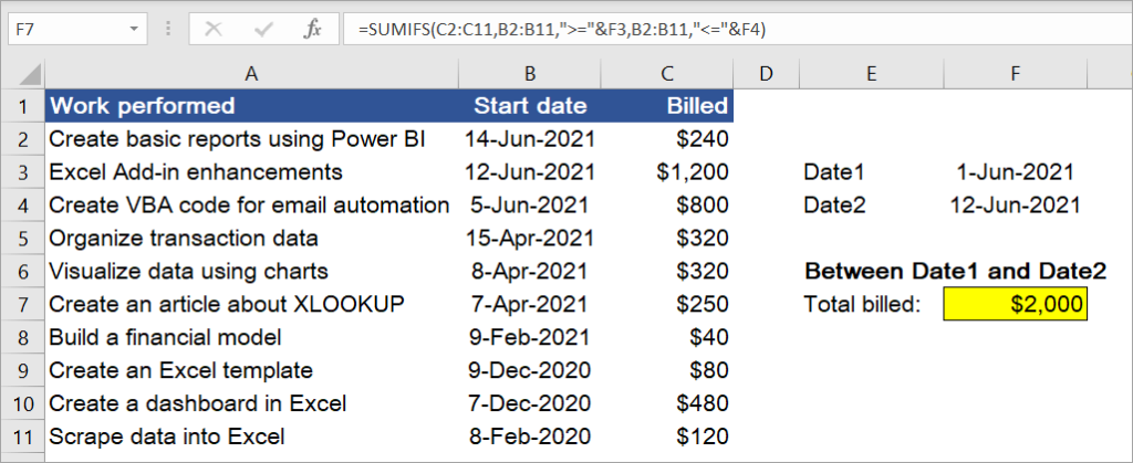
With the following data, suppose you want to sum the total bill for works started between 1-Jun-2021 (cell F3) and 12-Jun-2021 (cell F4). Use the formula below:

=SUMIFS(C2:C11,B2:B11,">="&F3,B2:B11,"<="&F4)

• 

#13: Excel SUMIF by month

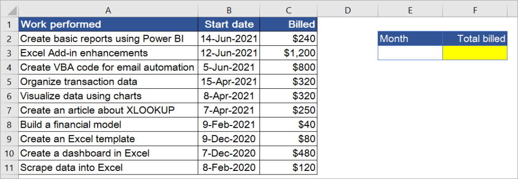
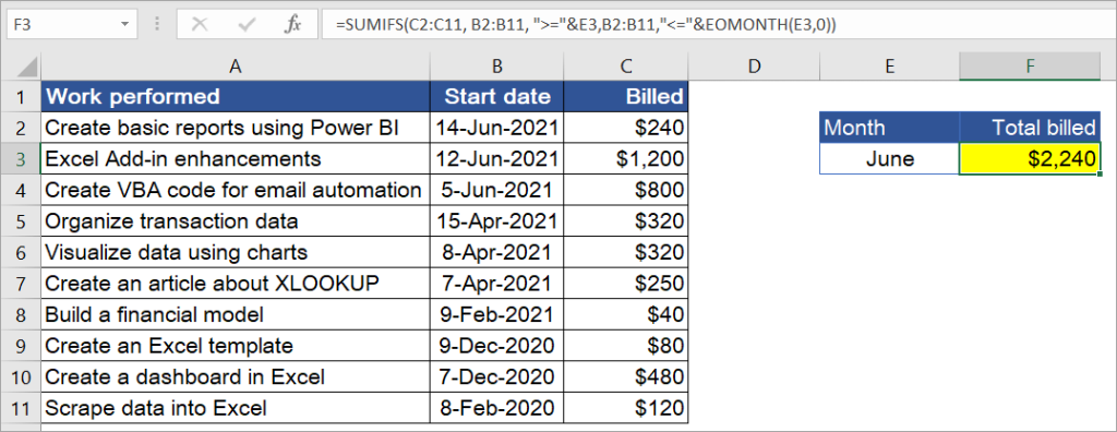
Suppose you have the following table and want to find the total bill for works that started in June 2001. To get the result, you can use a SUMIFS function with these two criteria: start dates >= first day of June AND start dates <= last day of June.

• 

Follow the steps below:

Step 1: Type the first date of June 2021 in E3.

• 

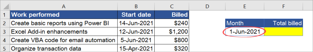
Step 2: Change the format of E3 to “mmmm” to display the month name.

• 

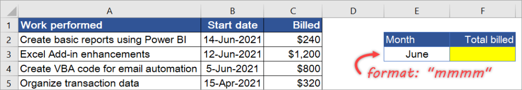
Step 3: Write the following formula to F3, then press Enter. Note: The EOMONTH function helps you to find the last day of the month.

=SUMIFS(C2:C11, B2:B11, ">="&E3,B2:B11,"<="&EOMONTH(E3,0))

• 

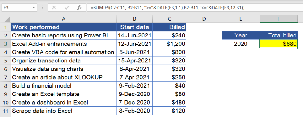
#14: Excel SUMIF by year

Still using the same data with the previous example, suppose you want to find the total bill for works that started in 2020. To get the result, use SUMIFS with these two criteria: start dates >= first day of 2020 AND start dates <= last day of 2020.

=SUMIFS(C2:C11, B2:B11, ">="&DATE(E3,1,1),B2:B11,"<="&DATE(E3,12,31))

• 

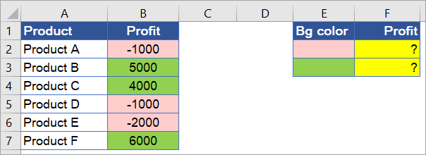
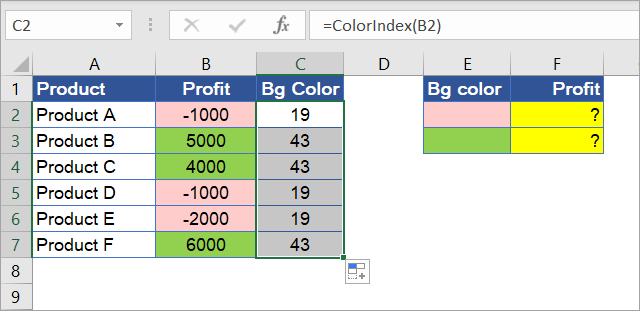
#15: Sum values based on background color

Suppose you have the following profit/loss data and want to sum based on the background color. In Excel, there is no default function to do that. But you can create an Excel VBA function to return the color index of a cell, and then use that index as the criteria in SUMIF.

• 

Follow the steps below:

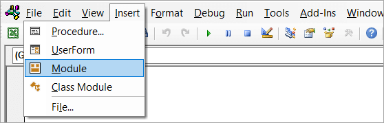
Step 1: Press Alt+F11 to open the Visual Basic Editor (VBE).

Step 2: Click Insert > Module.

• 

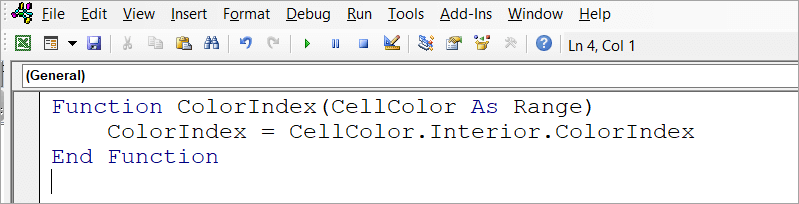
Step 3: Copy-paste the following function to the editor:

Function ColorIndex(CellColor As Range)
    ColorIndex = CellColor.Interior.ColorIndex
End Function

• 

Step 4: Type “Bg Color” as the header of column C. Then, type =ColorIndex(B2) in C2 and copy the formula down to C7.

• 

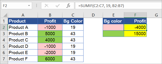
Step 5: Use SUMIF to calculate the total profit based on the background color, as follows:

• Formula in F2:

=SUMIF(C2:C7, 19, B2:B7)

• Formula in F3:

=SUMIF(C2:C7, 43, B2:B7)

• 

Read our guide on Excel SUMIFS VBA.

#16: Excel SUMIF to sum across multiple sheets

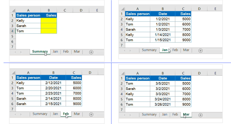
Suppose you have identical ranges in separate worksheets and want to summarize the total in the first worksheet, as shown in the following screenshot:

• 

To do that, you can use the SUMIF function with INDIRECT, wrapped in SUMPRODUCT. 

See the below steps to calculate the summary for the first salesperson (Kelly):

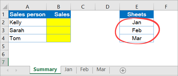
Step 1: List all the sheet names that are going to be summed in the Summary sheet. For example, in E2:E4 as shown below:

• 

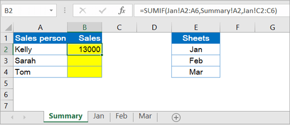
Step 2: Write a SUMIF formula for one sheet only – for example, Jan.

=SUMIF(Jan!A2:A6,Summary!A2,Jan!C2:C6)

• 

Step 3: Nest the formula inside SUMPRODUCT.

=SUMPRODUCT(SUMIF(Jan!A2:A6,Summary!A2,Jan!C2:C6))

Step 4: Replace the sheet reference with a list of sheet names. In this case, 

• Replace Jan!A2:A6 with INDIRECT("'"&E2:E4&"'!"&"A2:A6")
• Replace Jan!C2:C6 with INDIRECT("'"&E2:E4&"'!"&"C2:C6")

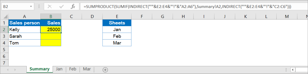
The complete formula will be:

=SUMPRODUCT(SUMIF(INDIRECT("'"&E2:E4&"'!"&"A2:A6"),Summary!A2,INDIRECT("'"&E2:E4&"'!"&"C2:C6")))

• 

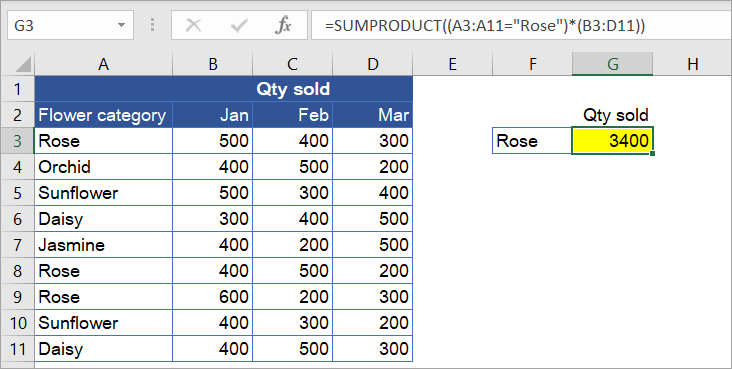
#17: Sum multiple columns using one criteria

With the following data, suppose you want to calculate how many roses were sold in three months — Jan, Feb, and Mar. You can’t use either SUMIF or SUMIFS in this case. One alternative is to use the SUMPRODUCT function, as follows:

=SUMPRODUCT((A3:A11="Rose")*(B3:D11))

• 

The first expression checks the range A3:A11 and returns an array of TRUE and FALSE. If any cell equals “Rose“, it will return TRUE, otherwise FALSE: 

{TRUE;FALSE;FALSE;FALSE;FALSE;TRUE;TRUE;FALSE;FALSE}

The result above is then multiplied by the values in range B3:D11:

{500,400,300;400,500,200;500,300,400;300,400,500;400,200,500;400,500,200;600,200,300;400,300,200;400,500,300}

The SUMPRODUCT function will calculate the following values, which finally returns 3400.

=SUMPRODUCT({500,400,300;0,0,0;0,0,0;0,0,0;0,0,0;400,500,200;600,200,300;0,0,0;0,0,0})

Limitations of the Excel SUMIF function

After looking at these examples, we are sure you have your own conclusion about the limitations of the SUMIF function. But anyway, here’s the summary:

• You can’t use Excel SUMIF with multiple AND criteria. SUMIF is designed to handle one criteria only. As shown in example #10, you can use SUMIF + SUMIF for multiple OR conditions. However, you can’t use it with multiple AND criteria. For this case, use SUMIFS instead.
• You can’t use Excel SUMIF to sum multiple columns at once. As demonstrated in example #17, you can’t use either SUMIF and SUMIFS to sum multiple columns using one criteria. One of the solutions is to use the SUMPRODUCT function.
• You can’t use Excel SUMIF with an array as its range argument. In example #11, you can see that SUMIF accepts an array in its criteria argument. However, for its range argument, SUMIF requires a cell range. Because of this, you can’t use a formula that returns an array in its range argument — here’s an example:

Suppose you have the following table and want to sum the total bill for works that started in 2020; you can’t use this formula: 

=SUMIF(TEXT(B2:B11,"yyyy"),"2020",C2:C11)

• 

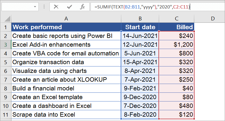
Why? That’s because the TEXT function in the above formula will return an array, which SUMIF doesn’t support. 

What to do when your Excel SUMIF function is not working

There are times when you’ll find that your SUMIF formula in Excel is not working, or returns inaccurate results. There can be many reasons for that. Most of them have to do with incorrect ranges and defining criteria incorrectly. Thus, we recommend checking the following points:

• Check the order of the arguments used in the formula. For example, if you use three arguments, remember the first argument is the range that contains criteria, not the range you want to sum. You might have confused this with the SUMIFS formula.
• Check the range of cells you use, especially if you copy-pasted the formula from another cell. These include the range you want to sum as well as the range that contains the criteria.  
• Ensure that you use double quotation marks (“”) for any criteria other than numeric.  
• Check the format of the values involved in the calculation. For example, if you sum values with the time format, ensure you use the correct time format for your range values and the result cells. 
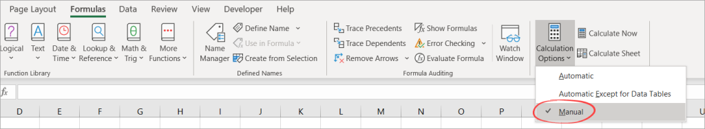
• You are sure that you’ve written the correct formula. Still, when you update the sheet, the SUMIF function doesn’t return the updated value? Well, in this case, check the formula calculation option in your spreadsheet. If it’s set to manual, press the F9 key to recalculate the sheet.  

• 

Finally, you’ve learned about the SUMIF function, including what it is, its syntax, how to use it, and its differences with SUMIFS. We also have covered various examples, as well as what to do when your function is not working. 

We hope this article helped you, but if it didn’t, let us know if you have any comments or suggestions in the comments section below.

Back to Blog