The COUNTIF function allows you to count the number of cells that meet a specific condition. It’s one of Excel’s most useful functions for data calculations and analysis. This blog post will show you how to use COUNTIF Excel VBA and provide some examples. Read on for all the details!
Excel VBA: COUNTIF function
COUNTIF is a function that counts the number of cells based on the criteria you specify. It combines COUNT and IF, and allows you to put in one criterion when doing the count. You can use this function, for example, to quickly get the number of products in a particular category, to find how many students scored higher than 80, and so on.
You can simply use COUNTIF in a cell’s formula by entering =COUNTIF(range, criteria). We have a helpful article that explains how to use Excel COUNTIF in a worksheet — so if you ever need a refresher, just give it a read!
In some cases, however, you may need to write VBA COUNTIF function as a part of automation tasks in Excel. Let’s say, every day, you need to automatically import data from multiple external sources, process the data, summarize it using COUNTIF and other statistical functions, and finally send a report in PDF or Powerpoint. Automating that process using VBA is a great way to improve productivity and save time!
Tip: As a shortcut for getting data from multiple sources into Excel, use Coupler.io. It’s a data integration solution to automate data load from over 60 cloud apps to Excel. These include Google Analytics, different ad platforms, Xero & QuickBooks, and so on. You can set up an integration with Excel with just a few clicks and save hours of your time. Try it right away for free! Select the desired source app in the form below and follow the in-app instructions to load data to Excel.
VBA COUNTIF syntax and parameters
COUNTIF is an Excel worksheet function. To write this function in VBA, specify the function name prefixed by WorksheetFunction, as follows:

As you can see in the above image, COUNTIF returns Double and has two required arguments:
| Name | Data type | Description |
| Arg1 | Range | Range. The range of cells to count. |
| Arg2 | Variant | Criterion. The criterion that defines which cells will be counted. It can be a number, text, expression, or cell reference. For example: 85, “red”, “<=50”, or D8. |
You can use the wildcard characters (? and *) in COUNTIF for more flexible criteria. This can be helpful if you want to do partial matching. For example:
- If you want to count all cells that contain the word “Jade” or “Jane,” you can use “Ja?e” as the criteria. A question mark matches any single character.
- If you want to count all cells that contain the word “Jake”, “James”, or “Jaqueline”, use “Ja*” as the criteria. An asterisk matches any sequence of characters.
- If you want to count all cells that contain “90” or “90*”, use “90~*” as the criteria. A tilde (~) followed by a wildcard character matches the character.
COUNTIF VBA Excel: Download an example file
You can download the following Excel file to follow along with the examples in this article:
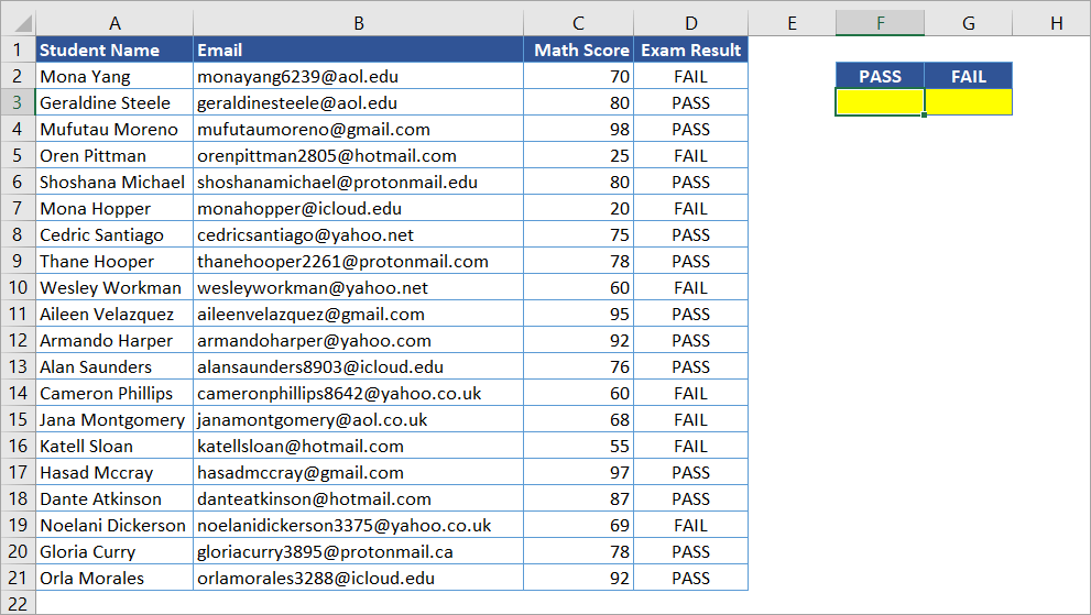
The file contains a list of students and their scores on a Math exam. After adding VBA codes, save it as a macro-enabled workbook (.xlsm).
How to use COUNTIF in VBA: A basic example
With the following student data, suppose you want to find how many students have passed vs. failed the math exam.
The following steps show you how to create a Sub procedure (macro) in VBA to get the result using VBA Excel COUNTIF:
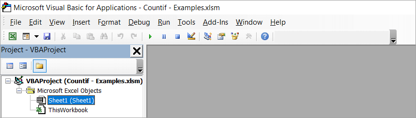
- Press Alt+11 to open the Visual Basic Editor (VBE). Alternatively, you can open the VBE by clicking the Visual Basic button on the Developer tab.
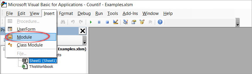
- On the menu, click Insert > Module.
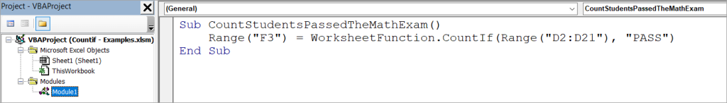
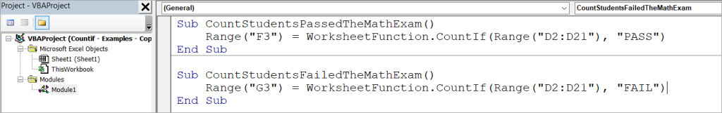
- To get how many students passed the exam, type the following Sub in Module 1. The code counts the cells in the range D2:D21 if the value equals PASS. Then, it outputs the result in F3.
Sub CountStudentsPassedTheMathExam()
    Range("F3") = WorksheetFunction.CountIf(Range("D2:D21"), "PASS")
End Sub
- Run the Sub by pressing F5. Then, check your worksheet — in cell F3, you should see the result:

- Now, add the following Sub in the module to get the number of students who failed their math exam. The code counts the cells in range D2:D21 if the value equals FAIL. It outputs the result in G3.
Sub CountStudentsFailedTheMathExam()
    Range("G3") = WorksheetFunction.CountIf(Range("D2:D21"), "FAIL")
End Sub
- Run the code again by pressing F5, then check your worksheet. In cell G3, you should see the result:
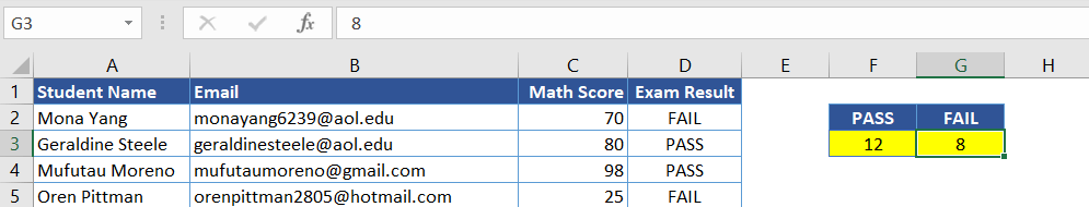
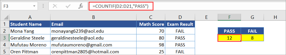
As you can see, the results of both Subs in F3 and G3 are values, not formulas. This makes the results not change if any of the values in range D2:D21 change. If you’d like to see formulas in the cells, you can write the code slightly differently, as shown in the below Subs:
Sub CountStudentsPassedTheMathExam2()
    Range("F3") = "=COUNTIF(D2:D21,""PASS"")"
End Sub

Sub CountStudentsFailedTheMathExam2()
    Range("G3") = "=COUNTIF(D2:D21,""FAIL"")"
End Sub
Here’s an example result in F3:
COUNTIF function VBA: More examples
There are many ways to use COUNTIF VBA Excel. We’ll take a look at examples with operators, wildcards, multiple criteria, and more.
COUNTIF VBA example #1: Using operators
Operators (such as >, >=, <, <=, and <>) can be used in COUNTIF’s criteria. For example, you can use the “>” operator to only count cells that are higher than a certain value.
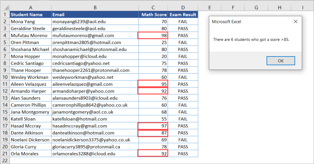
The following COUNTIF VBA code counts the number of students who got a score higher than 85:
Sub CountIfScoreHigherThan85()
    Dim rng As Range
    Dim criteria As Variant
    Dim result As Double

    Set rng = Range("C2:C21")
    criteria = "85"

    result = WorksheetFunction.CountIf(rng, ">" & criteria)

    MsgBox "There are " & result & " students who got a score higher than " & criteria & "."
End Sub
The code above uses three variables with different data types. First is rng, which stores the range of cells to count. The second is criteria, which holds the criteria we want to specify. The last is result, which stores the output of the COUNTIF function.
In this case, we are counting the cells in the range C2:C21 where its value is higher than 85. We use the “>” operator and combine it with the criteria using an ampersand symbol. The calculation result is stored in the result variable. Finally, the code outputs a message box showing the result:
COUNTIF VBA example #2: Using wildcards for partial matching
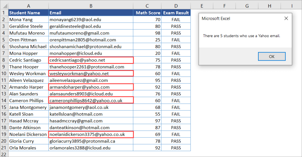
The following COUNTIF in VBA counts the students who use Yahoo emails:
Sub CountIfEmailIsYahoo()
    Dim rng As Range
    Dim criteria As Variant
    Dim result As Double

    Set rng = Range("B2:B21")
    criteria = "Yahoo"

    result = WorksheetFunction.CountIf(rng, "*" & criteria & "*")

    MsgBox "There are " & result & " students who use a " & criteria & " email."
End Sub
The function uses the “*” symbol at the beginning and end of the criteria to match all emails containing a Yahoo address. Notice that the criteria are not case-sensitive.
Here’s the output:
COUNTIF VBA example #3: Multiple OR criteria
You can use multiple COUNTIFs (COUNTIF+COUNTIF+…) for multiple OR criteria in one column. For example, you could use COUNTIFs to count the number of cells that contain “red” OR “blue.”
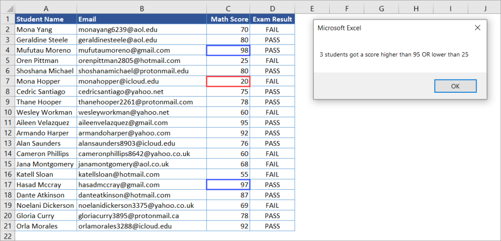
With our student dataset, you can use the following code to see how many students got scores higher than 95 OR lower than 25:
Sub CountIfMultipleOrCriteria()
    Dim rng As Range
    Dim criteria1, criteria2 As Variant
    Dim result As Double

    Set rng = Range("C2:C21")
    criteria1 = 95
    criteria2 = 25

    result = WorksheetFunction.CountIf(rng, ">" & criteria1) _
                + WorksheetFunction.CountIf(rng, "<" & criteria2)

    MsgBox result & " students got a score higher than " & criteria1 & " OR lower than " & criteria2
End Sub
The solution is simple and straightforward. You can just use multiple COUNTIFs if you have more than one OR criteria in a single column.
Here’s the output of the above code:
Pro tip: If you find yourself frequently performing this type of analysis with data from external systems, consider setting up an automated data pipeline with Coupler.io. This allows you to schedule regular imports from sources like Google Sheets, Airtable, or your CRM systems directly into Excel, where your VBA COUNTIF functions can automatically process the fresh data. This approach is particularly valuable for recurring reports or dashboards that need regular updates.
COUNTIF VBA example #4: Multiple AND criteria
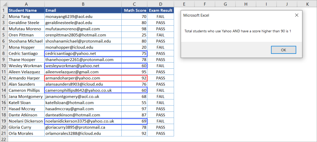
Suppose you need to count the number of students who use Yahoo email AND have a math score higher than 90. COUNTIF does not work in this case.
The COUNTIFS function might be the solution you’re looking for. You can also get the result manually using a loop, but we recommend you use COUNTIFS if possible.
Code 1: Using COUNTIFS
In the code below, we use the COUNTIFS function with 4 parameters: 2 range and 2 criteria parameters.
Sub CountIfsMultipleAndCriteria()
    Dim rng1, rng2 As Range
    Dim criteria1, criteria2 As Variant
    Dim result As Double

    Set rng1 = Range("B2:B21")
    criteria1 = "Yahoo"

    Set rng2 = Range("C2:C21")
    criteria2 = 90

    result = WorksheetFunction.CountIfs(rng1, "*" & criteria1 & "*", rng2, ">" & criteria2)

    MsgBox "Total students who use " & criteria1 & _
        " AND have a score higher than " & criteria2 & " is " & result
End Sub
Here’s the output:
Code 2: Manually count in a loop
The below code loops from Row 2 to 21 and checks all values in Column B and Column C. If there is a match, the result variable is incremented by 1. For Column B, the Like operator is used to find a partial match. Notice that it’s case-sensitive, so we apply LCase when making the comparison.
Sub CountWithMultipleAndCriteria()
    Dim criteria1, criteria2 As Variant
    Dim result As Double

    criteria1 = "Yahoo"
    criteria2 = 90
    result = 0

    ' Loop each row
    For i = 2 To 22
        If LCase(Cells(i, "B")) Like LCase("*" & criteria1 & "*") _
          And Cells(i, "C") > criteria2 Then
            result = result + 1
        End If
    Next i

    MsgBox "Total students who use " & criteria1 & _
        " AND got a score higher than " & criteria2 & " = " & result
End Sub
There might be a time when you might want to do processing in a loop. For example, if you’re trying to count cells by checking if they’re bold or having certain colors, etc., which can’t be done using COUNTIFS alone.
COUNTIF VBA example #5: Using COUNTIF to highlight duplicates
There are times when you have large amounts of data with duplicates. Instead of using the Remove Duplicates command on the Data tab, you might want to just mark them for future reference. This is a pretty useful option when you’re doing data analysis.
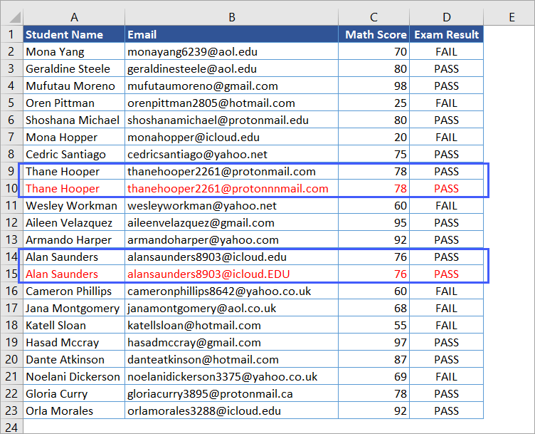
See the below code that uses Excel VBA COUNTIF to mark the duplicates with red color. The checking is based on Column A which contains student names. It leaves the first unique values unmarked.
Sub HighlightDuplicates()
    With Range("A2:D23")
        .Select
        .FormatConditions.Delete
        .FormatConditions.Add Type:=xlExpression, Formula1:="=COUNTIF($A$2:$A2,$A2)>1"
        .FormatConditions(1).Font.Color = RGB(255, 0, 0)
    End With
End Sub
If you insert two duplicates and run the above code, you’ll see a result similar to this below—duplicates are marked in red color:
Taking your data analysis beyond VBA
While VBA COUNTIF functions are powerful for analyzing data within Excel, many data analysis tasks involve working with information from external sources. For example, you might want to:
- Count customer interactions from your CRM system
- Analyze task completion rates from project management tools
- Track financial metrics from accounting software
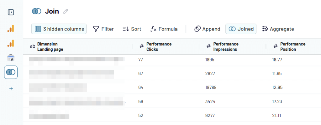
Instead of writing complex VBA code to import and process this data, you can use Coupler.io’s no-code data integration solution. Coupler.io automatically imports your data from various sources directly into Excel, where you can then apply your COUNTIF functions for analysis. Moreover, it allows you to prepare the dataset on the go using filters, aggregations, data join, and custom formulas!
For instance, you could set up a daily automatic import of your sales data, then use the COUNTIF examples we’ve covered to track metrics like:
- Number of sales over a certain threshold
- Count of deals by sales representative
- Identifying duplicate customer entries
This approach combines the power of VBA analysis with the convenience of automated data imports.

Automate data flows to Excel with Coupler.io
Get started for freeCOUNTIF in VBA Excel – Summary
With Excel VBA, you can use the COUNTIF function to tally up numbers based on the criteria you set. After reading this article, hopefully, you can easily use this function in VBA code for things like data analysis and calculations.
If you’re looking for a solution to import data from various sources into Excel without having to code any VBA code, consider using Coupler.io. You can also use it to automate your reporting process by scheduling the imports. Check out our website for more information about how Coupler.io can help you take your data analysis to the next level.
Thanks for reading, and happy COUNTing!
