The VLOOKUP function only returns a single match. And what if a lookup value has multiple matches within a range? Let’s see the options you have.
How to VLOOKUP for multiple matches
We imported a dataset from Google Sheets to Excel using Coupler.io, a solution for automatic data exports from multiple apps and sources. You can easily load your data from over 70 cloud sources as well. Just select the needed tool in the form below and click Proceed to get started for free.
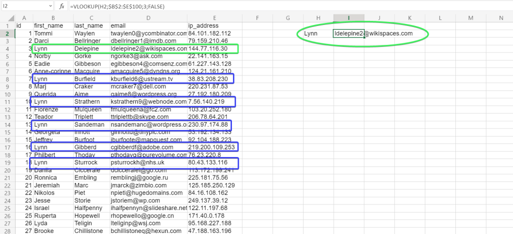
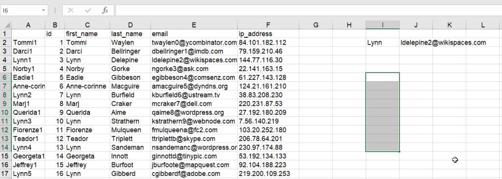
Now we need to lookup email addresses for a user with the name “Lynn“. The VLOOKUP formula only returns one match, whereas there are a few.
Read more about Microsoft Excel integrations for data export on a schedule.
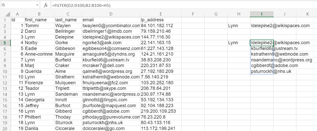
The best way to lookup all the matches is the FILTER function, which is available for Excel Online and Excel for Microsoft 365.
Other Excel users will have to use a workaround to return all the matches, but it is still possible.
Excel FILTER function
Syntax
=FILTER(array,include,[if_empty])array– the range or array to filter.include– filter criteria.if_empty– the optional parameter to return when no results meet the criteria.
In our example, the FILTER formula to return multiple values will look as follows:
=FILTER(D2:D100,B2:B100=H5)
If for any reason you can’t or don’t want to go with Excel Online or Excel 365, you’ll need to tinker with the following workaround.
VLOOKUP for multiple results (workaround)
The logic of this workaround is the following:
- Step 1: Create a separate column where we will create unique strings for our lookup value, such as Lynn1, Lynn2, Lynn3, etc. This will let us differentiate lookup values.
- Step 2: Look up these unique strings to return matching values.
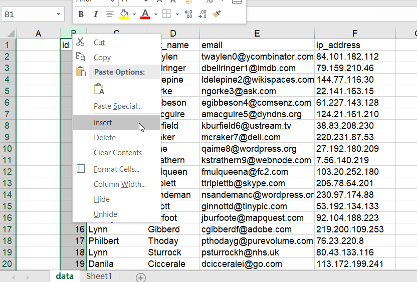
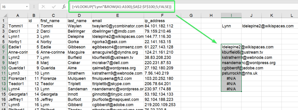
Step 1: Create a column with unique strings for the lookup value
Insert a column to the left of your dataset like this:
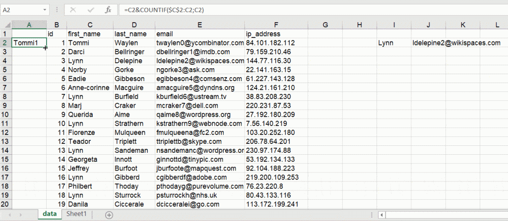
Insert the following COUNTIF formula in the A2 cell and drag it down:
=C2&COUNTIF($C$2:C2,C2)
Note: Unfortunately, we can’t apply an array formula for this.
Step 2: VLOOKUP formula for multiple values
Now we can insert a VLOOKUP formula to return all the matching results for our lookup value:
=VLOOKUP("Lynn"&ROW(A1:A100),$A$2:$F$100,5,FALSE)
"Lynn"&ROW(A1:A100)– a formula, which will generate a unique string to be used as a lookup value, such as Lynn1, Lynn2, Lynn3, etc.$A$2:$F$100– the range to look up5– the column to return the matching values from
Do not forget about the method of applying array formulas in Excel desktop:
- Select an array for the VLOOKUP formula
- Insert the formula to the formula bar and press Ctrl+Shift+Enter for Windows (Command+Return for Mac)
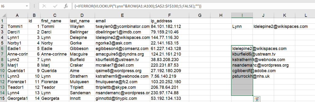
To get rid of #N/A, let’s nest our VLOOKUP formula with IFERROR as follows:
=IFERROR(VLOOKUP("Lynn"&ROW(A1:A100),$A$2:$F$100,5,FALSE),"")
Now it looks better:
As we mentioned earlier, Coupler.io allows you to import data from over 70 data sources to Excel, including platforms like Facebook Ads, Google Analytics 4 (GA4), HubSpot, and Shopify. You can easily consolidate data from multiple sources in Excel, without needing to download CSV files from each platform.

Automate data import to Excel with Coupler.io
Get started for free