Do you struggle with date formats in Google Sheets? Cases could be different from simply displaying ‘February’ instead of ‘2’ to fixing the broken date formulas.
This guide is created to help you overcome any struggles related to Google Sheets date format. You will learn how to format dates, set up custom formats, juggle date functions, and many more. Let’s go!
How to format dates in Google Sheets
There are two ways to format dates in Google Sheets – manually via the UI and using date functions.
To explain each option, we imported datasets from Clockify, Harvest, and other sources to Google Sheets using Coupler.io for free. It’s a reporting automation solution that allows you to connect your data source to Google Sheets and other destinations. Another benefit of this tool is that you can set up a schedule to refresh data automatically.
Check it out yourself: just select the needed data source and click Proceed to load data from it to your spreadsheet.
Format dates in Google Sheets manually
In the following dataset, let’s change the format of data in column J from yyyy-mm-dd into mm/dd/yyyy.
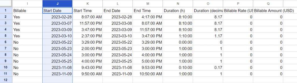
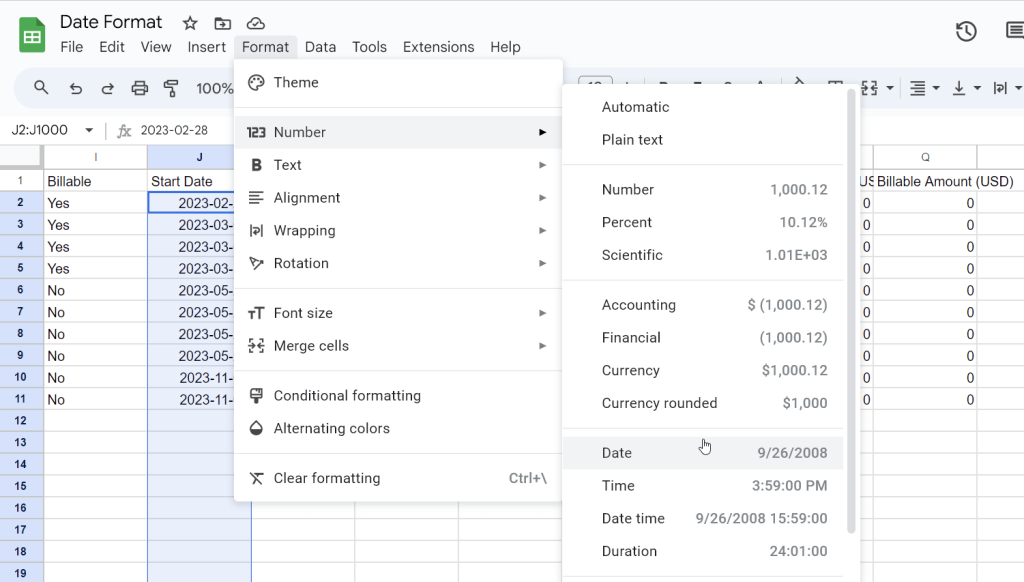
For this, select the range (J2:J11) or entire column and go to Format ? Number ? Date.
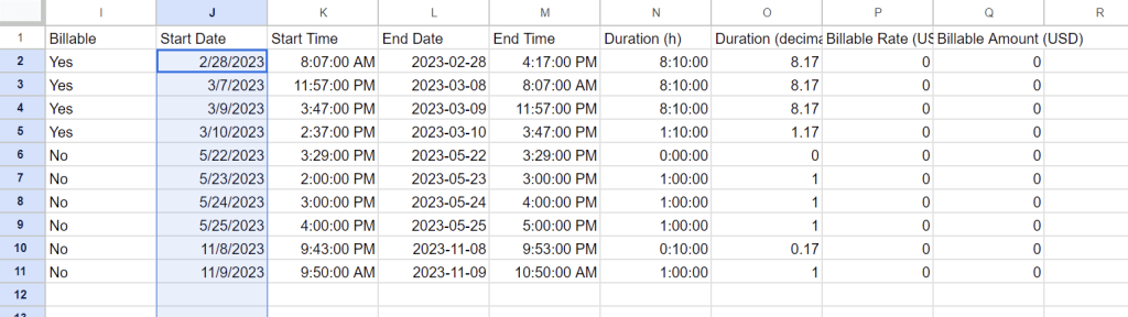
That’s it:)
Format dates in Google Sheets using functions
In Google Sheets, there are multiple date functions to format values in date or date-time format, and perform other date-centered manipulations. For example, the DATE function returns a date value of the specified year, month, and date values.
The EDATE function returns a date based on the provided start date and the number of months before or after it. Here is a table with the date functions available in Google Sheets.
| Name+Description | Syntax |
|---|---|
| DATE Converts a provided year, month, and day into a date. Learn more | =DATE(year, month, day) |
| DATEDIF Calculates the number of days, months, or years between two dates. | =DATEDIF(start_date, end_date, unit) |
| DATEVALUE Converts a provided date string in a known format to a date value. | =DATEVALUE(date_string) |
| DAY Returns the day of the month that a specific date falls on, in numeric format. | =DAY(date) |
| DAYS Returns the number of days between two dates. | =DAYS(end_date, start_date) |
| DAYS360 Returns the difference between two days based on the 360-day year used in some financial interest calculations. | =DAYS360(start_date, end_date, [method]) |
| EDATE Returns a date a specified number of months before or after another date. | =EDATE(start_date, months) |
| EOMONTH Returns a date representing the last day of a month which falls a specified number of months before or after another date. | =EOMONTH(start_date, months) |
| HOUR Returns the hour component of a specific time, in numeric format. | =HOUR(time) |
| ISOWEEKNUM Returns the number of the ISO week of the year where the provided date falls. | =ISOWEEKNUM(date) |
| MINUTE Returns the minute component of a specific time, in numeric format. | =MINUTE(time) |
| MONTH Returns the month of the year a specific date falls in, in numeric format. | =MONTH(date) |
| NETWORKDAYS Returns the number of net working days between two provided days. | =NETWORKDAYS(start_date, end_date, [holidays]) |
| NETWORKDAYS.INTL Returns the number of net working days between two provided days excluding specified weekend days and holidays. | =NETWORKDAYS.INTL(start_date, end_date, [weekend], [holidays]) |
| NOW Returns the current date and time as a date value. | =NOW() |
| SECOND Returns the second component of a specific time, in numeric format. | =SECOND(time) |
| TIME Converts a provided hour, minute, and second into a time. | =TIME(hour, minute, second) |
| TIMEVALUE Returns the fraction of a 24-hour day the time represents. | =TIMEVALUE(time_string) |
| TODAY Returns the current date as a date value. | =TODAY() |
| WEEKDAY Returns a number representing the day of the week of the date provided. | =WEEKDAY(date, [type]) |
| WEEKNUM Returns a number representing the week of the year where the provided date falls. | =WEEKNUM(date, [type]) |
| WORKDAY Calculates the end date after a specified number of working days. | =WORKDAY(start_date, num_days, [holidays]) |
| WORKDAY.INTL Calculates the date after a specified number of workdays excluding specified weekend days and holidays. | =WORKDAY.INTL(start_date, num_days, [weekend], [holidays]) |
| YEAR Returns the year specified by a given date. | =YEAR(date) |
| YEARFRAC Returns the number of years, including fractional years, between two dates using a specified day count convention. | =YEARFRAC(start_date, end_date, [day_count_convention]) |
| EPOCHTODATE Converts a Unix epoch timestamp in seconds, milliseconds, or microseconds to a datetime in Universal Time Coordinated (UTC). | =EPOCHTODATE(timestamp, [unit]) |
In this section, we will only focus on five date functions: TODAY, DAY, MONTH, YEAR, and DATE.
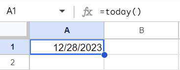
Google Sheets TODAY function
TODAY returns the current date on a cell – keep in mind that the date inserted in this way will auto-update.
Syntax:
=TODAY()Example:
Google Sheets DAY function
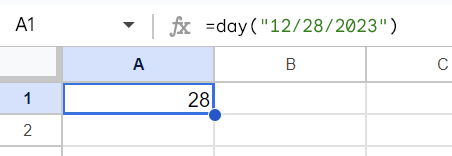
DAY returns the day from a given date.
Syntax:
=DAY(date)Example:
=day("12/28/2023")
Google Sheets MONTH Function
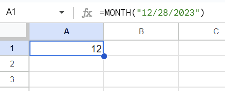
MONTH returns the month from a given date.
Syntax:
=MONTH(date)Example:
=month("12/28/2023")
Google Sheets YEAR Function
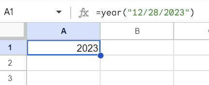
YEAR returns the year from a given date.
Syntax:
=YEAR(date)Example:
=year("12/28/2023")
Google Sheets DATE function
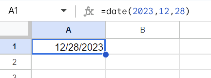
DATE converts a provided year, month, and day into a date. Because we use the US location, the date format is MM/DD/YYYY.
Syntax:
=DATE(year, month, day)Example:
=date(2023,12,28)
How to create a sheet with a specific date format in Google Sheets
The date format specific to your Google Sheets spreadsheet is affected by the specific regional date format you choose. For example:
- specific date format in the United States is MM/DD/YYYY
- specific date format in Europe is DD/MM/YYYY
- specific date format by ISO 8601 is YYYYMMDD or YYYY-MM-DD
- specific date format in Japan is YYYY/MM/DD
- and so on.
To choose one specific date format, you need to set up your Location in spreadsheet settings. We have explained how you can do this in this section below.
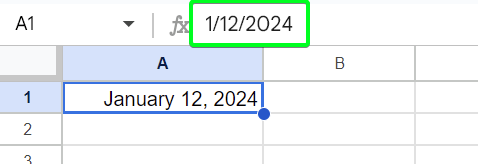
For example, the date format specific to the United States is MM/DD/YYYY. This means that the date January 12, 2024, should look like this: 1/12/2024.
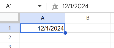
If you enter this date in another format, for example, 12/1/2024, Google Sheets will recognize it as text rather than date.
How to set up custom date format in Google Sheets
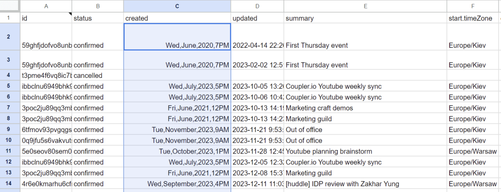
Let’s say you have a list of events imported from Google Calendar to Google Sheets. You want to create a custom date format for the created column that will show day, month, year, and time like this: Wed, June, 2023, 7PM
You can customize the format by yourself with the following steps:
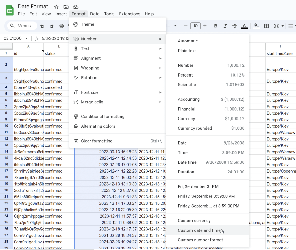
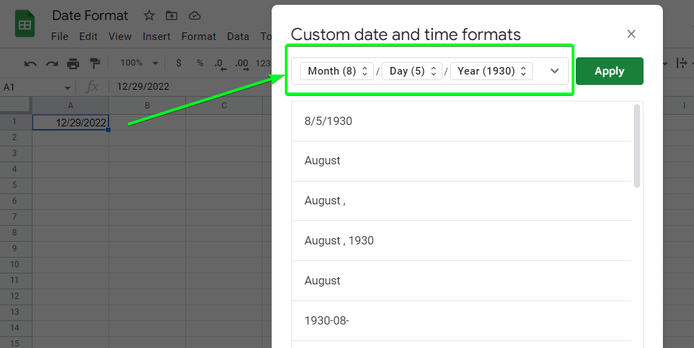
- Select the column range C2:C and go to Format ? Number ? Custom date and time
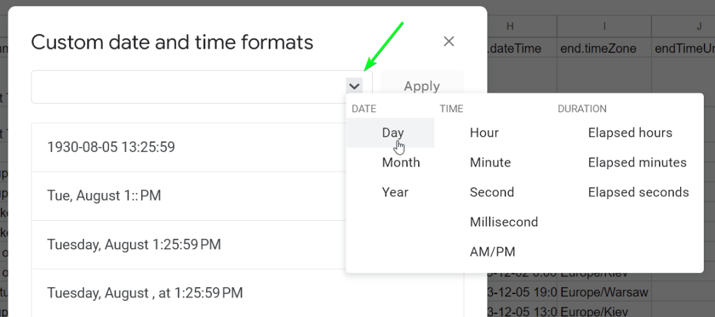
- When the custom date and time formats dialogue appears, find the date format by scrolling down the page. In my case, I didn’t find any option that would meet my requirement on the date format. So, I will create a custom one by adding, editing, or removing the format components. To add components, you need to click this drop-down arrow.
For my custom date formate I did the following
- Added a day as an abbreviation and separated it with a comma
- Added a month as full name and separated it with a comma
- Added a full numeric year and separated it with a comma
- Added hour without leading zero
- Added full AM/PN component
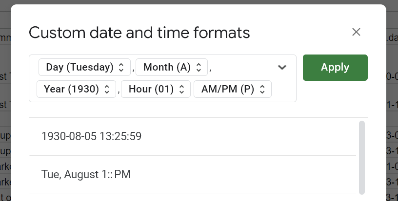
Once you’re ready, click Apply and there you go!
How to convert a date as month or year in Google Sheets?
If you need to convert the date into the month or year value only in Google Sheets, you can use MONTH, and YEAR functions.
Convert month value using the MONTH function
The MONTH function in Google Sheets is a function that returns the month number from a given date. The syntax is =MONTH(date).
For example, suppose we have a date 12/29/1993, which we need to convert into the month value. Use this syntax to extract the year
=MONTH(12/29/1993)
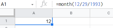
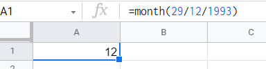
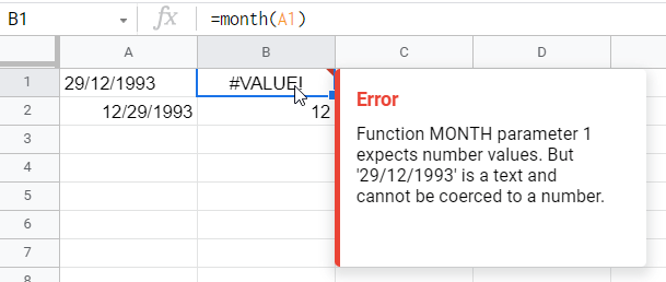
You can use different date formats as the parameter for the MONTH function. For example, 29/12/1993 will work.
But if you reference another cell in your MONTH formula, then make sure that this cell contains a date value. Otherwise, the formula will return an error.
Convert year value using the YEAR function
The logic of the YEAR function is the same – it extracts the year value from a given date. The syntax is =YEAR(date). But, the date specified can be:
- a cell reference to a cell containing a date
- a function returning a date type
- a number
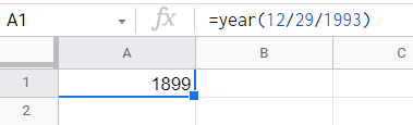
So, if you use just 12/29/1993 in your YEAR formula, it will return a wrong value.
But if you use a proper parameter in your formula, it will work:
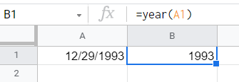
Just like with the MONTH function, make sure that the cell you reference to in your YEAR formula contains a date value. Otherwise, the formula will return an error.
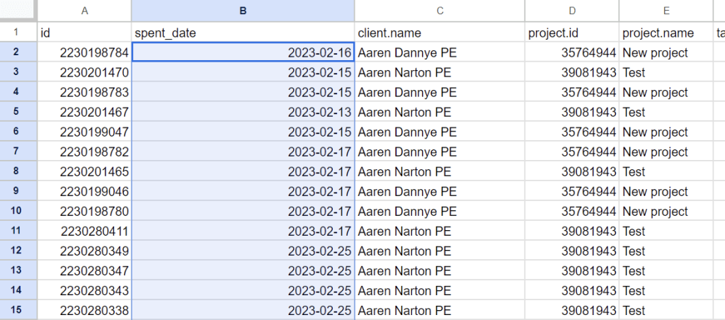
How to validate a date format in Google Sheets with pop-up alert
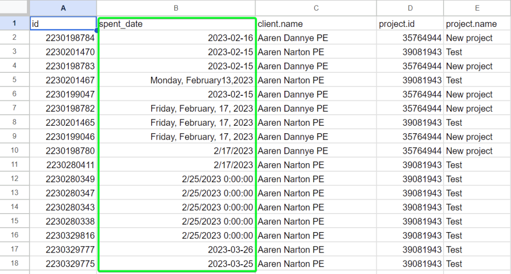
If you use automated data entry in Google Sheets, you’ll likely have no issues related to incorrect date format. However, if you and your team mates enter data manually, this problem can happen pretty often. Here is what it may look like:
To avoid this situation, you need to do Data validation to control the date format you and your team can input. Do the following steps:
- Select the entire column B and apply the default date format for it, for example, yyyy-mm-dd. For this, go to Format > Number > Custom date and time. Select the needed format and apply it.
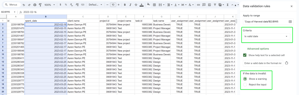
- Now go to Data ? Data Validation. Click +Add rule and select Is a valid date as Criteria. In the Advanced options, you need to check Reject input in the section If the data is invalid.
Optionally, you can check the Show help text for a selected cell and provide help text, for example, “Enter a valid date in the format mm-dd-yyyy“. Click Done.
Once this data validation rule is enabled, you and your colleagues won’t enter the incorrect date format. You’ll be able to select a date from a drop-down calendar.
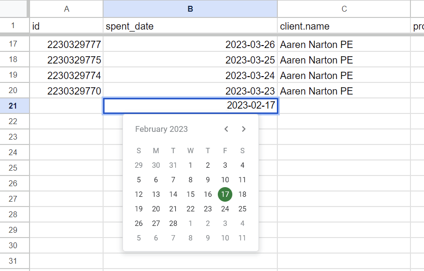
And even if someone copies and pastes date in incorrect format, it will still be shown in the format you’ve set up.
How to change date format in Google Sheets
To change date format in Google Sheets:
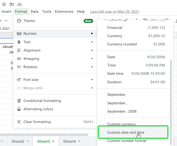
- Open the Format menu on the Google Sheets toolbar and select Number.
- Scroll down a bit to the Custom date and time
- Select the predefined format or make it yourself.
Let’s see how this works in practice.
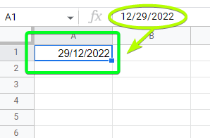
How to change date format in Google Sheets to dd/mm/yyyy
Let’s change the date from the US format to the European one:
12/29/2022 into 29/12/2022
- Select the cell with the date value, then go to Format => Number => Custom date and time. You’ll see the current date format.
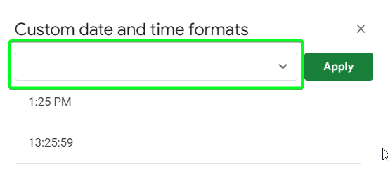
- Scroll down to find the necessary date format. In our case, we did not find the one we need. So, let’s make it. For this, clear the current date format. You can use the Backspace button for this.
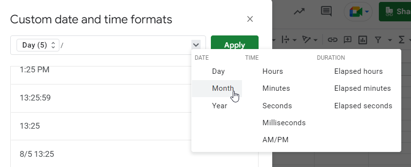
- Then use the drop-down arrow to add the necessary values in the required order: dd/mm/yyyy. Do not forget to add slashes between the values.
- Once your custom date format is ready, click Apply.
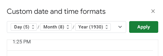
There you go!
How to change back the default date format in Google Sheets
To change the date format to the default date format of Google Sheets (MM/DD/YYYY), you need to do the following:
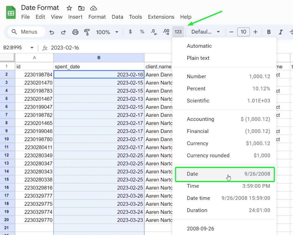
- Select a column or cells with date values and go to Format ? Number ? Date
The selected cells changed the date to default.
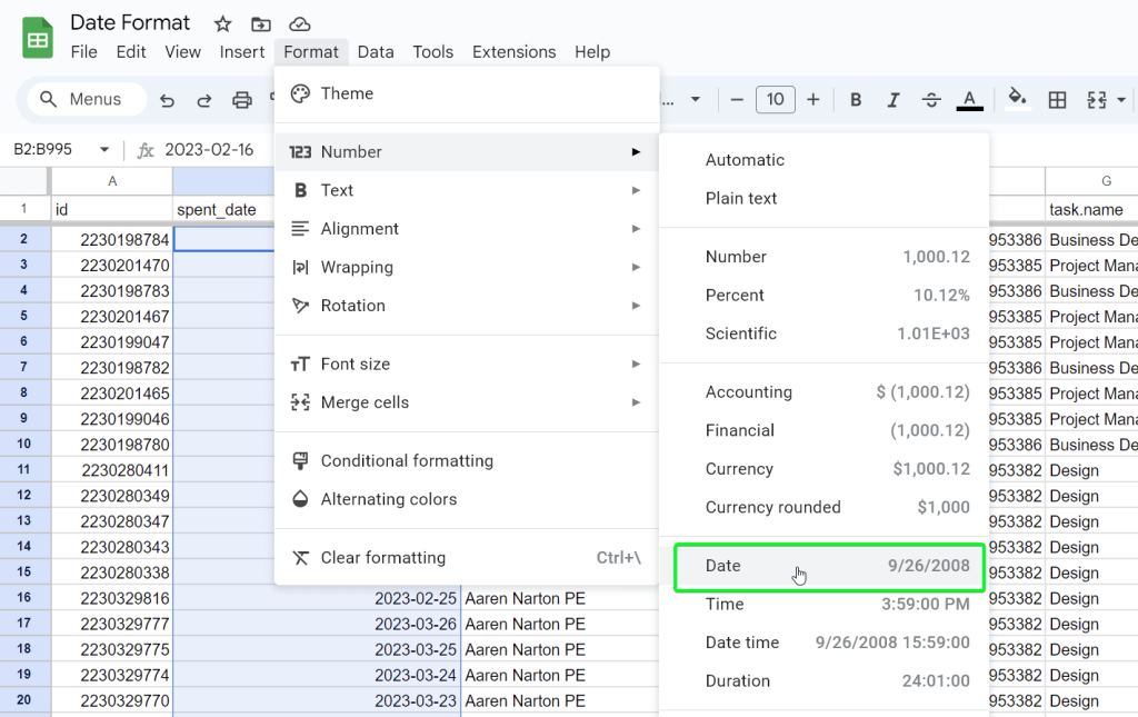
Tips You can use a shortcut “123” button in the top menu bar, then select Date.
How to set a date in Google Sheets based on a conditional format
If you want to highlight cells that meet certain criteria, conditional formatting is the best answer. This helps you better understand spreadsheets at a glance and create spreadsheets that are more human-readable by your whole team. Let’s check out several use cases.
How to highlight dates in a range, row, or column if the date is today’s date
How to highlight dates in a range
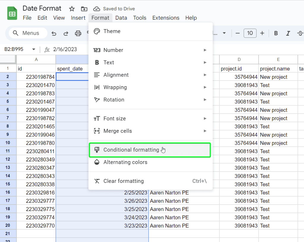
- Select the range of cells, click Format ? Conditional formatting (or right-click => View more cell actions => Conditional formatting)
- Customize your conditional format rules as follows:
- Under Format cells if… select Date is then select exact date if you want to highlight cells containing an exact date. You can specify the exact date or a date formula.
- You’ll need also to choose the formatting style for the cells that meet your criteria. Here is what it looks like when we specified the date: 2/15/2023.
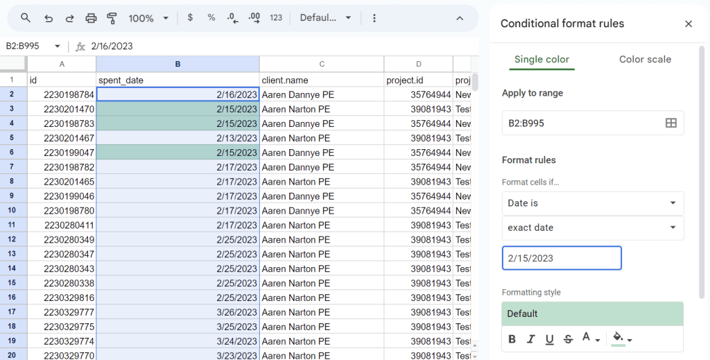
In addition to the exact date options, you can select today, tomorrow, yesterday, in the past week, in the past month, and in the past year.
How to highlight dates in a row
Basically, you need to do pretty much the same as above to highlight dates in a row. The only difference is that you have to select a row of cells containing date values.
Highlight dates in a column
Here also, all you have to do is adjust which column you want to highlight at the first step, such as select the entire column A, then repeat the flow above.
How to highlight an entire row with specified dates
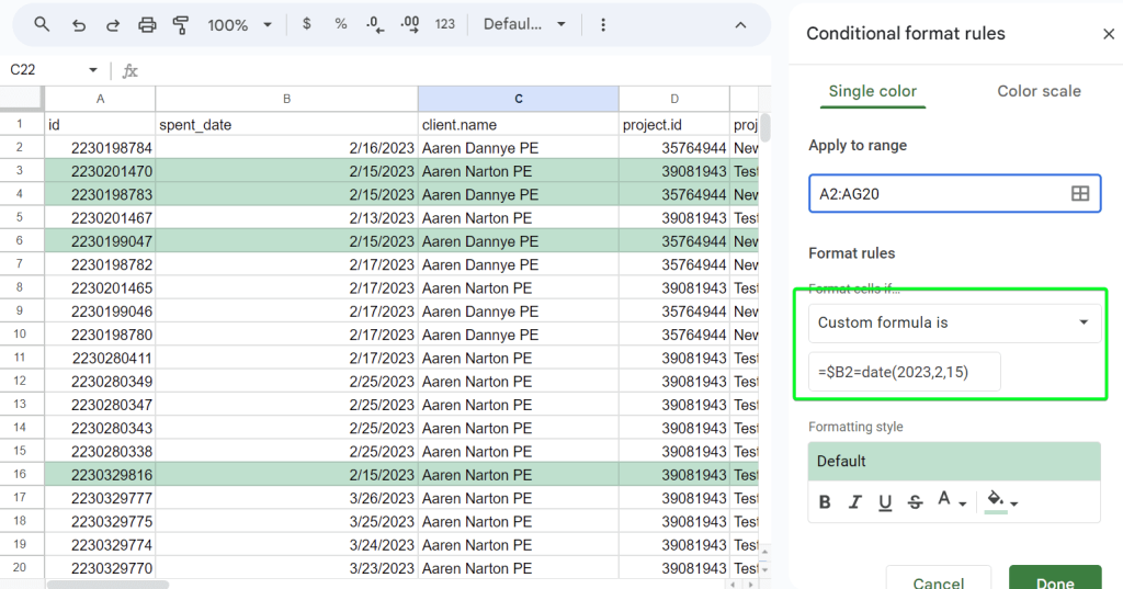
Let’s say, you want to highlight an entire row that contains the date 2/15/2023. Complete the following steps:
- Select all the cells on a sheet except for the title row. Then go to Format ? Conditional formatting (or right-click => View more cell actions => Conditional formatting)
- Customize your conditional format rules as follows:
- Under Format cells if… select Custom formula is and use the following formula:
=$B2=date(2023,2,15)- Choose the formatting style for your highlighting.
How to highlight weekends in Google Sheets using conditional format
You have a set of date values and you wonder which of them are weekends? Let’s see how you can highlight weekends using conditional formatting:
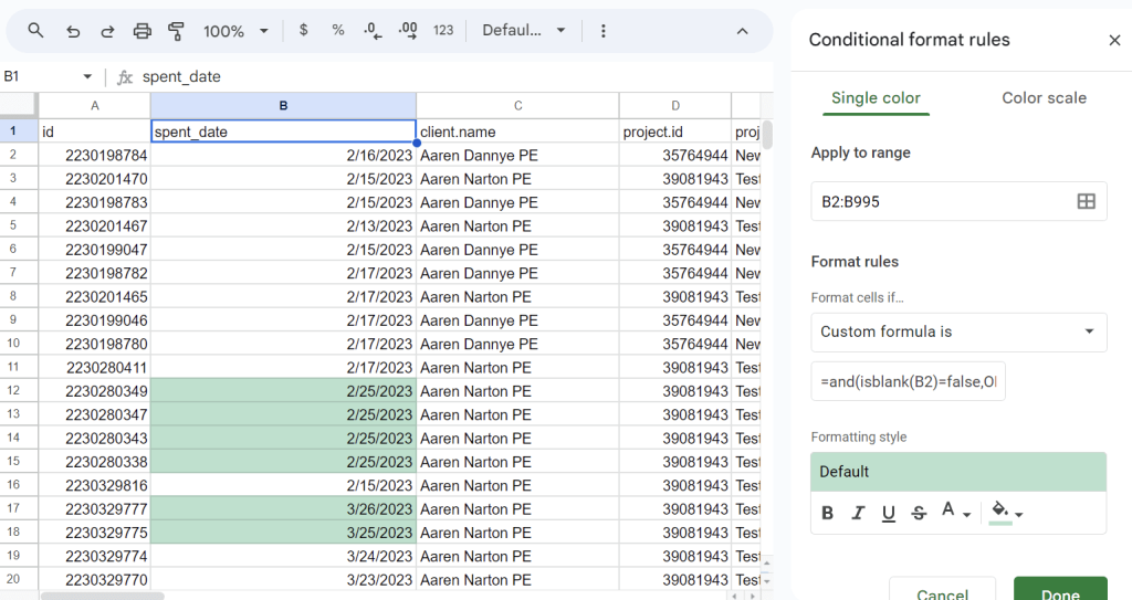
- Select the range of cells, click Format ? Conditional formatting (or right-click => View more cell actions => Conditional formatting)
- Customize your conditional format rules as follows:
- Under Format cells if… select Custom formula is and use the following formula:
=and(isblank(B2)=false,OR(weekday(B2)=7,weekday(B2)=1))- Choose the formatting style for your highlighting.
How to highlight specific weekdays in Google Sheets
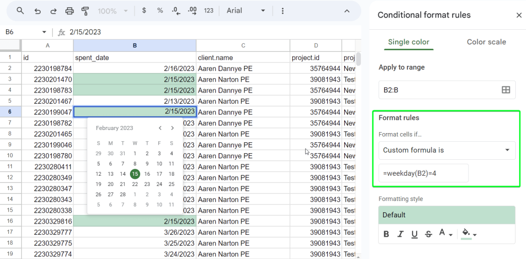
It’s clear that cells that have not been highlighted in the previous case are weekdays. But what if you need to highlight specific weekdays, for example, Wednesdays? The WEEKDAY function will help you do this:
- Select the range of cells, click Format ? Conditional formatting (or right-click => View more cell actions => Conditional formatting)
- Customize your conditional format rules as follows:
- Under Format cells if… select Custom formula is and use the following formula:
=weekday(B2)=4- Choose the formatting style for your highlighting.
Note:
The values of WEEKDAY are as follows:
- 1 = Sunday
- 2 = Monday
- 3 = Tuesday
- 4 = Wednesday
- 5 = Thursday
- 6 = Friday
- 7 = Saturday
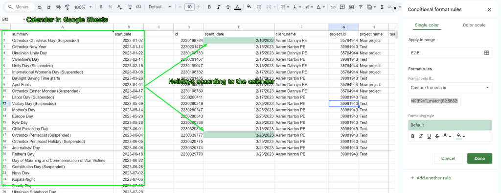
How to highlight a list of holidays in a calendar range in Google Sheets
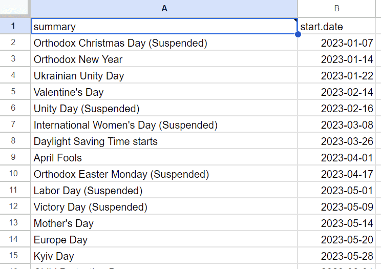
And what about holidays? Since they are different depending on your location, it makes sense to prepare your own calendar of holidays in Google Sheets. You can do this manually or load this data from your Google Calendar to Google Sheets. Here is what we have:
Now you can use this data for highlighting holidays in your dataset. Add it to your sheet with the dataset and follow the steps below:
- Select the range of cells, click Format ? Conditional formatting (or right-click => View more cell actions => Conditional formatting)
- Customize your conditional format rules as follows:
- Under Format cells if… select Custom formula is and use the following formula:
=IF(E2="",,match(E2,$B$2:$B,0))- Choose the formatting style for your highlighting.
Here is what we’ve got:
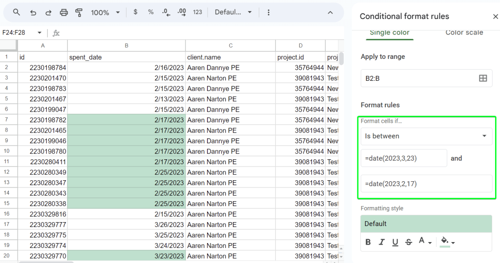
How to highlight the date if it falls between two dates
Suppose you want to highlight in green the date values in column A that fall between 3/23/2023 and 2/17/2023. Here are the steps:
- Select the range of cells, click Format ? Conditional formatting (or right-click => View more cell actions => Conditional formatting)
- Customize your conditional format rules as follows:
- Under Format cells if… select Is between. Two boxes will appear underneath. In the first box, enter this formula
=date(2023,2,17) - in the second box:
=date(2023,2,17) - Choose the formatting style for your highlighting.
- Under Format cells if… select Is between. Two boxes will appear underneath. In the first box, enter this formula
Here is what we’ve got:
How to highlight a column based on a date in another column
What if we have data in two columns, and want to highlight cells in column A if dates in column B are less than six months from today?
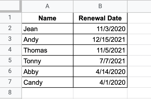
- Select the range (A2:B7).
- Click Format ? Conditional formatting.
- Customize your conditional format rules as follows:
- In the Conditional format rules box, Under Format cells if… select custom formula is.
- Copy this formula
=$B2<edate(today(),6)and paste in the Value or formula box. - Click the fill color and choose red.
- Click Done.
How to prevent Google Sheets from changing date format
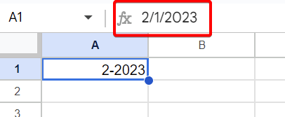
Sometimes you face a situation where a string is being interpreted as a date. For example, you enter “2-2022-1-2023″ automatically, as shown in the picture below:
To prevent data from being changed to date format in your spreadsheet, you need to preformat the cells or the entire column. To do this, select the needed cell range or a column and go to Format ? Number ? Plain text
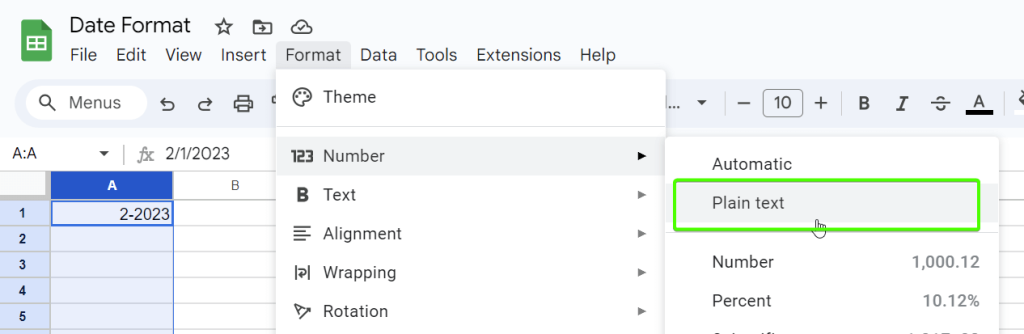
Now, all the numeric entries you’re making will not be automatically converted to a date.
How to automatically change format date in Google Sheets
To automatically convert a value to a date in your desired format, you can use the ARRAYFORMULA function as follows:
=arrayformula(IF(logical_test, [value_if_true], [value_if_false])). logical_testis a value or a given condition that is stored as Original Date-Time that can be evaluated as TRUE or FALSE.value_if_trueis the value to return as a new date format (DD MMMM YYYY) whenlogical_testevaluates to TRUE.value_if_falseis the value to return as blank whenlogical_testevaluates to FALSE.
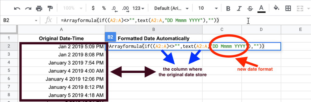
This formula can change the original date format into your target format. All you need to do is prepare another column to store your target format and set up an ARRAYFORMULA formula there to convert the original date format into your target date format automatically. Here is an example:
Suppose we have the Original Date-Time format in column A. We want to automatically change values from this column into the DD MMMM YYYY format (02 January 2019). The converted values will be stored in column B titled Formatted Date Automatically.
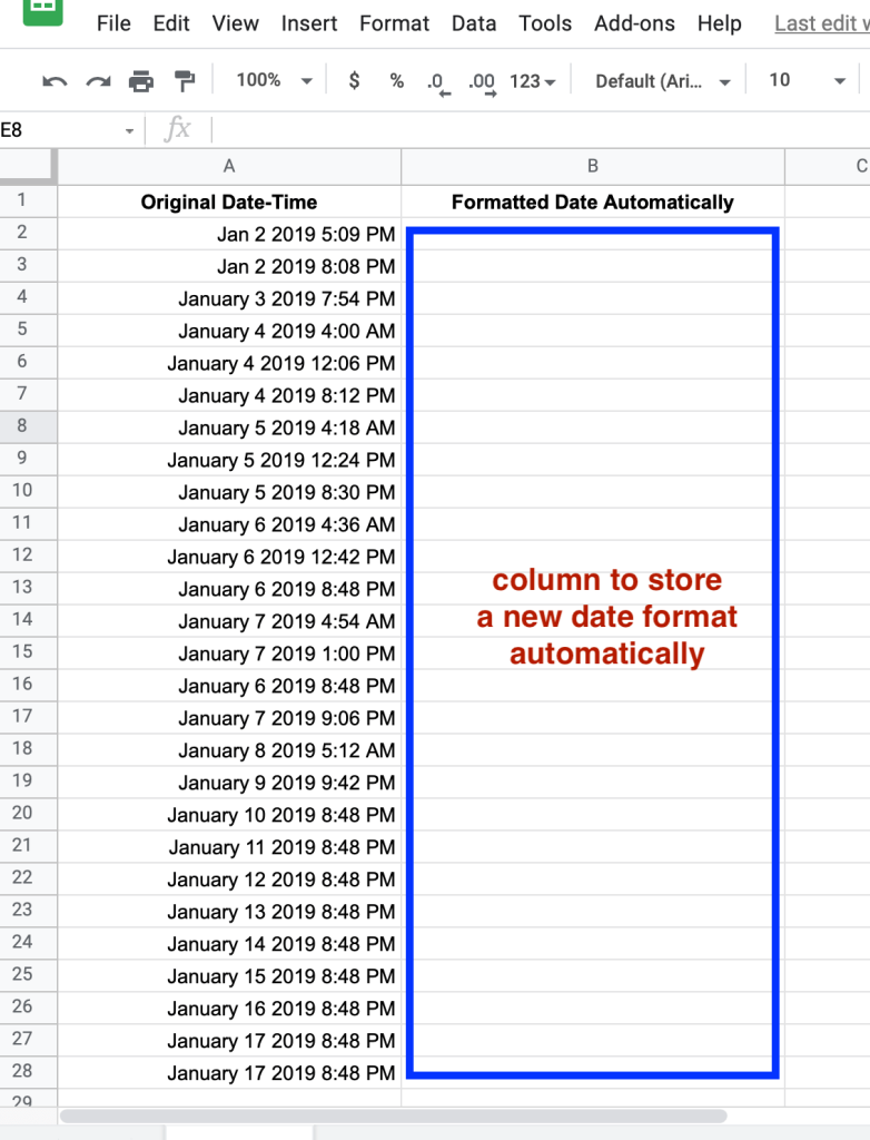
We need to apply the ARRAYFORMULA formula in Column B, so whenever we input the new date format into column A, this formula will change it into a targeted format automatically and will be stored in column B. Here is what the formula will look like:
=arrayformula(if((A2:A)<>"",text(A2:A,"DD mmmm YYYY"),""))
Remember that this formula may ignore the specific input date format of the Original Date-Time column if the date values do not correspond to your spreadsheet location format. For example, if you use the UK location, the formula will ignore 21 01 2019, but it will work with 01 21 2019.
Now, whatever date we input into column A, it will automatically change into DD MMMM YYYY in column B. The result test is:
Date time format FAQs to refresh your memory
What is the date format in Google Sheets?
The date format in Google Sheets is a standard way provided by Google Sheets to express a particular period of the day (D), month (M), and year (Y) in a numeric calendar date, which helps you eliminate ambiguity. Here is what day, month, and year can be written in Google Sheets:
| Day | Month | Year |
|---|---|---|
| In numbers (one or two digits) as the day of the month. Example: 2, 31 | In numbers (one or two digits) as the month in year. Example: 1, 12 | In two or four digits. Example: 24 or 2024. |
| Abbreviated day of the week (three digits) Example: Tue | Abbreviated month (three digits) Example: Apr | |
| Full name of the day. Example: Tuesday | Full name of the month. Example: April |
The separators you can use between the components are slash (/), dot (.), dash (-), and space ( ).
In Google Sheets, you have two high-level choices for date format:
- Use the default formats
Default formats here mean the default/specific date formats that are used in your region/country. Suppose you live in the UK, then the default date format that you can use is DD/MM/YYYY – 24/04/1997, for example.
- Create a custom format
With this choice, you are free to define the date format, as long as the format meets the criteria in Google Sheets. For example, after the date format MM-DD-YYYY, you want to add hh:mm as a two-digit number for the hour and a two-digit number for the minute – 04-15-2017 10:14 AM.
Date time formats in Google Sheets
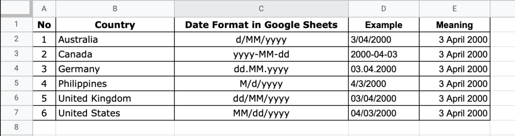
The date formats in Google Sheets vary all over the world, with different separations among them. Some people manipulate date formats into their spreadsheets in textual values such as “yesterday” or “Tuesday“, while others input in advanced formats such as “26/3/2001 02:05 PM“. There is also a cross-cultural audience that represents dates in different ways that could be incompatible with other audiences – for example in the United States, the date format is MM/DD/YYYY, while most of Europe uses DD/MM/YYYY. This difference could confuse people.
Below is the table of some countries that have different date formats in Google Sheets. For example, April 3, 2000 will look as 03.04.2000 for people in Germany and 04.03.2000 for the United States. Without the information that is written in column C, you would get confused because the date’s interpretation will be different between these countries.
To eliminate the ambiguity of the problem above, this article explains how to understand and apply various date formats in certain cases in Google Sheets. But first, please set your Google Sheets location.
Google Sheets location – what it is and why you need it
Google Sheets location is a setting in Google Sheets that controls how to enter number values (such as date-time values) into Google Sheets. This setting is what presets your Google Sheets date format based on your territory. For example, 18 August 2019 – if you’re in the US, the date format that will be put in your sheets is 08/18/2019, while in the UK, it will be 18/08/2019.
It’s crucial to have the correct location set to ensure you use the correct date formats, especially if the file that you import into your Google Sheets was created in another country that has a different date format.
To set up your spreadsheet location, follow the steps below:
- In the Google Sheets menu, click File ? Spreadsheet settings.
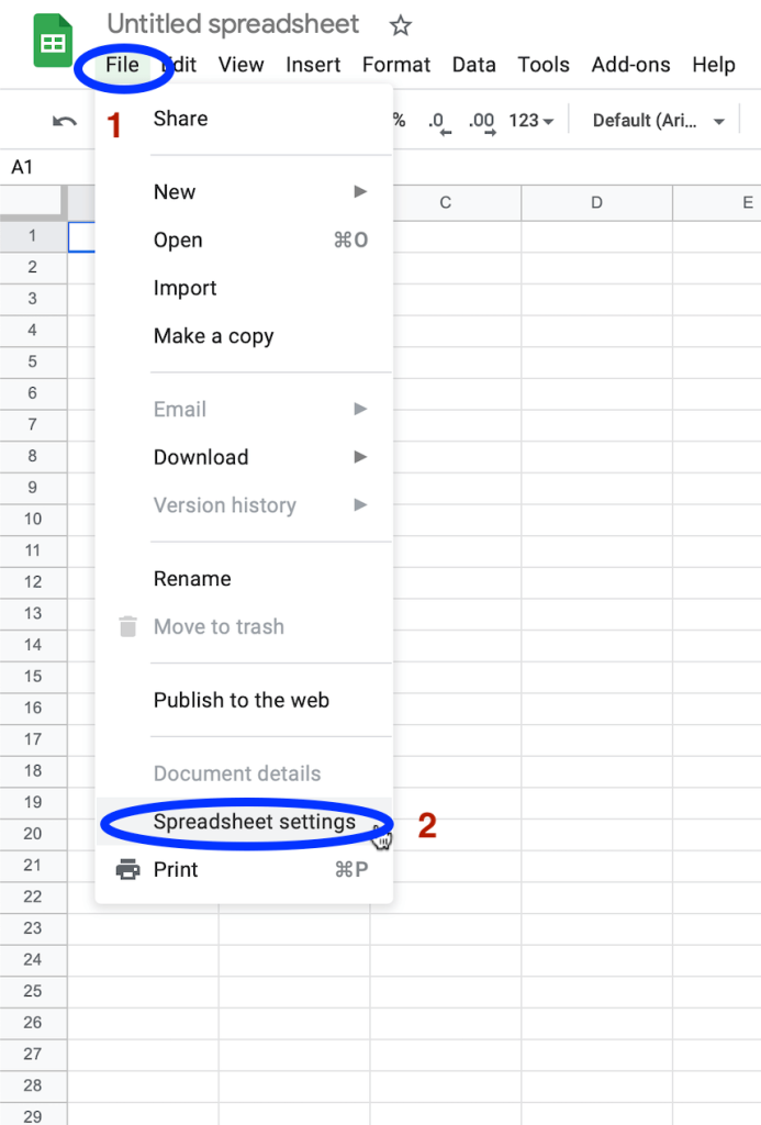
- Under the General tab, you will find Locale – pick the desired location from the drop-down list:
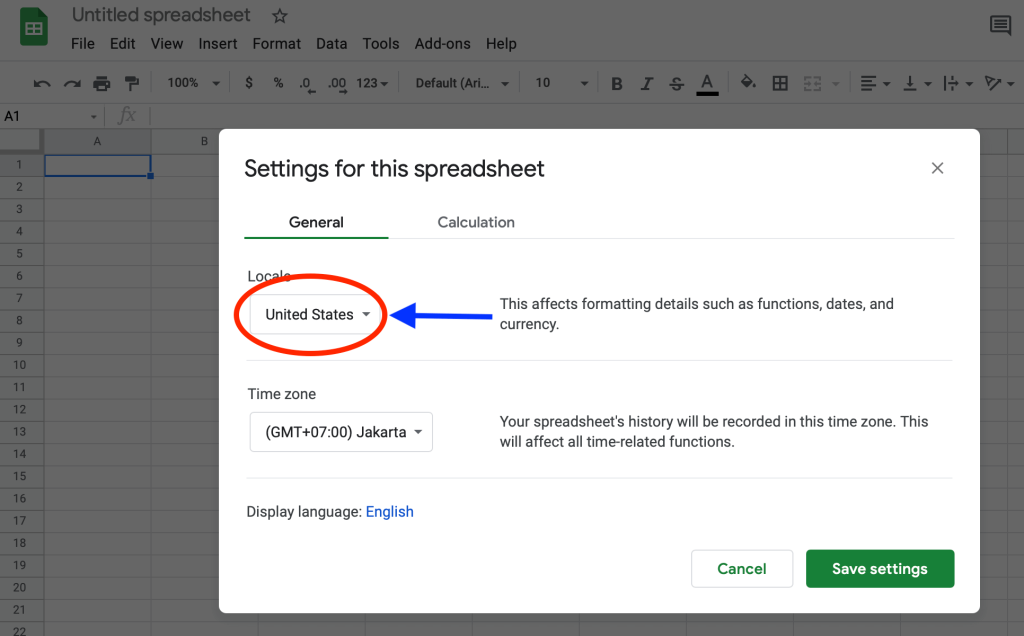
This Locale setting helps you ensure the correct date format using a regional standard date format. Now, you are ready to learn about using various date formats in Google Sheets.
What is a Google Sheets European date format
The European date format is dd/mm/year, for example, 17/07/2024.
It differs from the US date format in which the month value goes first – mm/dd/year, for example, 07/17/2024.
This difference causes confusion between citizens of the US and European countries. However, in Google Sheets, you can change the date format in different default and custom options. We’ll talk about this later.
If the Google Sheets date format doesn’t work
In some cases, you may find that Google Sheets date format is not compatible with your data. There are three reasons why this might be the case:
Incorrect syntax in your date functions
If you enter the parameters to your date function not in a numeric format, then it will return the #VALUE! error.
For details, let’s take a look at an example – a table containing Year in column A, Month in column B and Day in column C. We want to create a date format in MM/DD/YYYY (because we use the US location) using the DATE function combining Column A, B, and C using the syntax =date(year, month, day). The result is shown below:
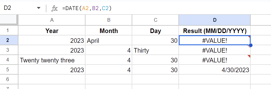
In D2, the error #VALUE! is returned because the parameter 2 (Month) is not a number but a string (April).
Likewise, if we input a string for Year or Day, #VALUE! will be returned as an error.
To fix this error, we should input all values in numbers. In D5, the correct input values are shown in A5, B5, and C5 so we get the correct result without errors.
Year values are less than 0 or greater than 10,000
Google Sheets will return the #NUM! error value if you type the year as less than 0 or greater than 10,000. Here is an example of the DATE formula.
=DATE(-100,4,3)
The same error will occur if you use a year value greater than 10,000:
=DATE(10000000,4,5)
Your input date value does not comply with your Google Sheets location setting
The date value you input will be treated as textual values if they are not in the format of your Google Sheets location setting.
For example, European date format (dd/mm/yyyy) is not recognized by Google Sheets if your location is set to the United States. The solution is to use the US date format (mm/dd/yyyy) or change your location settings.
It’s time to end this date topic with Google Sheets date formats. Hope you enjoy your stay 🙂