Excel files are also called workbooks for a very good reason. They can have multiple sheets, or worksheets, to help you organize your data. When working with multiple sheets, you may need to have links between them so that values in one sheet can be used in another.
In this article, we’ll explain how to link data between worksheets in Excel. You’ll see several examples of linking sheets in the same workbook as well as across different ones.
Problems with linking large data between worksheets in the same or different Excel workbooks
Indeed, using multiple worksheets can certainly make your data in one workbook easier to manage. However, linking large amounts of data between worksheets could decrease the performance of your Excel workbook. Avoid inter-workbook links unless it’s absolutely necessary because they can be slow, easily broken, and not always easy to find and fix.
We suggest you try another solution ?
When getting large data from different worksheets, especially from different workbooks, we recommend that you import instead of linking. Linking will slow down your Excel file, while an optimized performance can be maintained by simply importing the data. Use Coupler.io to refresh your data on the schedule you want to keep your data up-to-date.
1. Collect data
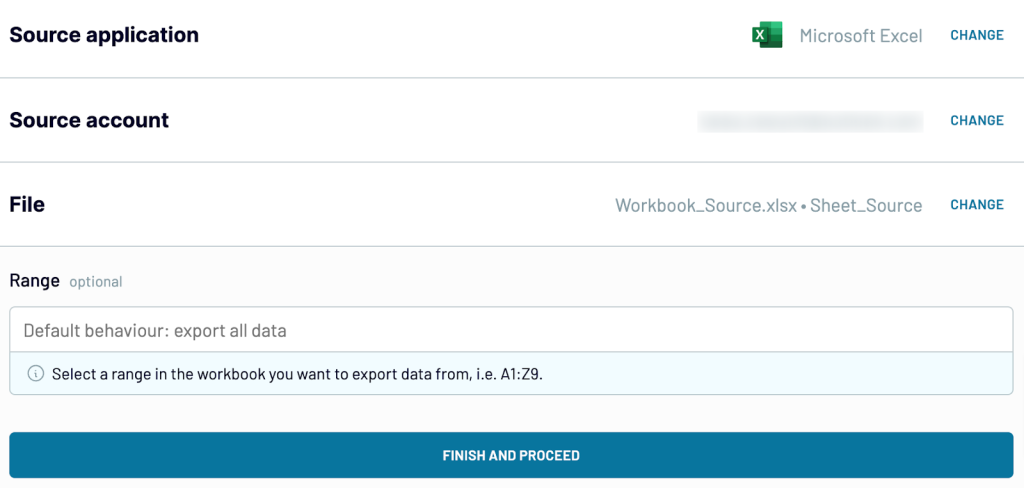
To start using Coupler.io, use the form below: click Proceed to sign up for a free account:
Connect to your Microsoft account and select the workbook and worksheet(s) you want to import. If you want, you can import only a selected range from your worksheets, e.g., range B3:G10 only.
2. Organize and transform data
Check the data you are going to export. In this step, you can:
- Rename, rearrange, hide, or add extra columns.
- Apply filters and sort data.
- Create new columns with custom formulas.
- Combine data from several accounts or from different apps.
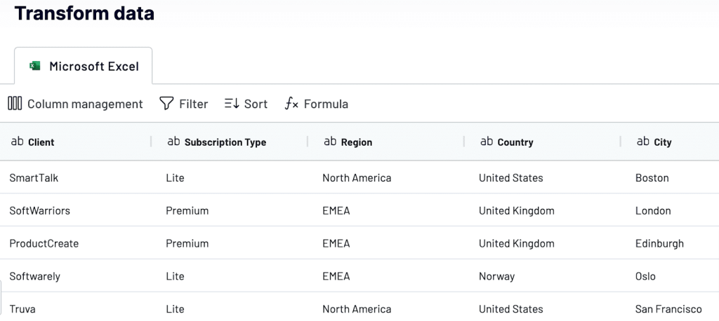
If your data looks correct, click Proceed.
3. Set up the destination
Choose the workbook and worksheet where you want your data to be imported.
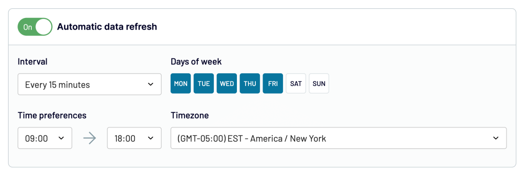
Toggle on the Automatic data refresh to schedule your data exports. You can specify an update interval from every month to every 15 minutes, making your report live.
Finally, click Run Importer to link the selected workbooks and automate data flow between them.
How to link two Excel sheets in the same workbook
Now, let’s see how to link two sheets in the same Excel workbook, including some tips and examples.
How to link sheets in Excel with a formula
To refer to a cell or range in another worksheet in the same workbook, type the name of the source worksheet followed by an exclamation mark (!) before the range address—see the following examples:
- To reference a single cell A1 in Sheet2:
=Sheet2!A1
- To reference a single cell A1 but the sheet name contains spaces:
='Sheet 2'!A1
- To reference a range of cells A1 to C10 in Sheet2:
=Sheet2!A1:C10
- To reference column A in Sheet2:
=Sheet2!A:A
- To reference multiple columns A to E in Sheet2:
=Sheet2!A:E
- To reference row 5 in Sheet2:
=Sheet2!5:5
- To reference multiple rows 1 to 5 in Sheet2:
=Sheet2!1:5
- To reference a worksheet-level named range Data in Sheet2:
=Sheet2!Data
- To reference a workbook-level named range Data in Sheet2:
=Data
You can always manually type the linking formula in a destination cell. However, doing that is not recommended because it typically leads to mistakes. So, instead of typing the formula manually, check the tips below.
Tip 1: Create a link from the destination sheet
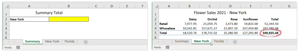
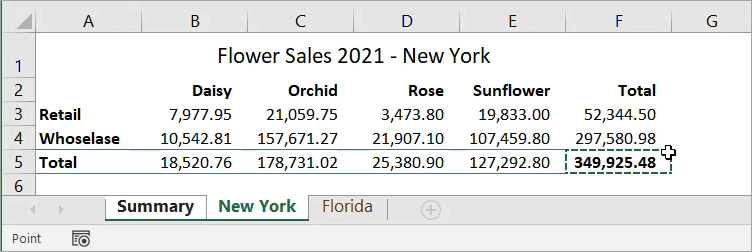
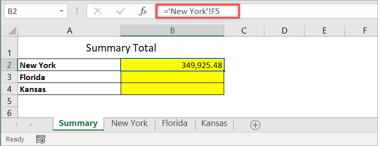
With the following spreadsheet, suppose you want to show the total for New York in the Summary sheet. In cell B2 of the Summary sheet, you want to display the values of cell F5 from the New York sheet.
To do that, follow the steps below:
- Begin by opening the destination sheet (Summary).
- Type = (equal sign) in the destination cell (B2).
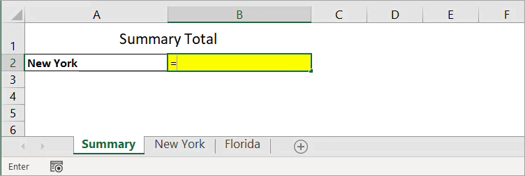
- Switch to the source sheet (New York).
- Select the cell you want to link (F5), then press Enter.
As a result, when you click on the destination cell, you’ll see the following formula:
='New York'!F5
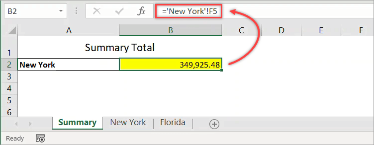
Notice that Excel automatically encloses the sheet name with single quotation marks because there is a space character in the sheet name.
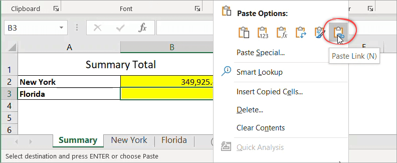
Tip 2: Use Copy and Paste Link
This second tip also allows you to link to another sheet without manually typing the linking formula. Unlike the first method which begins from the destination sheet, this method starts from the source sheet.
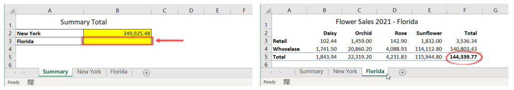
This time, suppose you want to show the total for Florida in the Summary sheet. In cell B3 of the Summary sheet, you want to display the values of cell F5 from the Florida sheet.
Follow the steps below:
- Begin by opening the source sheet (Florida).
- Right-click on the cell you want to link (F5), then select Copy.
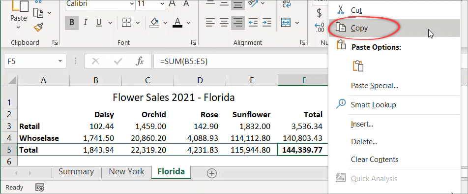
- Switch to the destination sheet (Summary).
- In the destination cell (B3), right-click and select Paste Link.
As a result, when you click on B3, you’ll see the following formula:
=Florida!$F$5
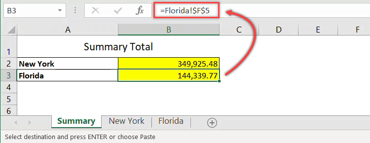
Notice that by default, this method returns an absolute reference. If you want to change it to a relative reference, simply highlight the formula and press F4 multiple times to remove the dollar signs.
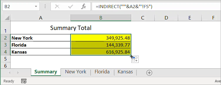
How to link numbers from different sheets in Excel using the INDIRECT function
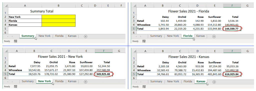
In the previous example, notice that the New York and Florida sheets have the same layout. In cases like this, you can also use the INDIRECT function in the formula to get the totals.
Now, let’s see the following spreadsheet with a Summary sheet and three other sheets with a similar layout. Assume you want to link the total in cell F5 from the three sheets and put them in the Summary sheet using the INDIRECT function.
To do that, follow the steps below:
- Link the total for New York only:
='New York'!F5
- Replace the formula using the INDIRECT function below. Notice that we concatenate A2 with single quotes because its value contains a space character.
=INDIRECT("'"&A2&"'!F5")
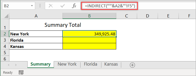
- Drag the formula down to A4 to apply it to the other states.
How to link data in a range of cells between sheets in Excel
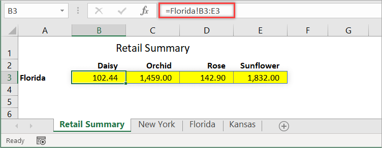
With the following spreadsheet, suppose you want to link the retail sales data for Florida and put them in the Retail Summary sheet, as the following screenshot shows:
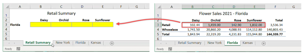
The range to link is in B3:E3 of the second sheet. To display it in the destination sheet, use the following formula in a cell:
=Florida!B3:E3
How to link columns from different sheets to another sheet in Excel
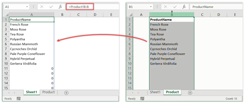
With the following spreadsheet, suppose you want to link the entire Column B from the Product sheet to Sheet1. To do that, you can use the following formula:
=Product!B:B
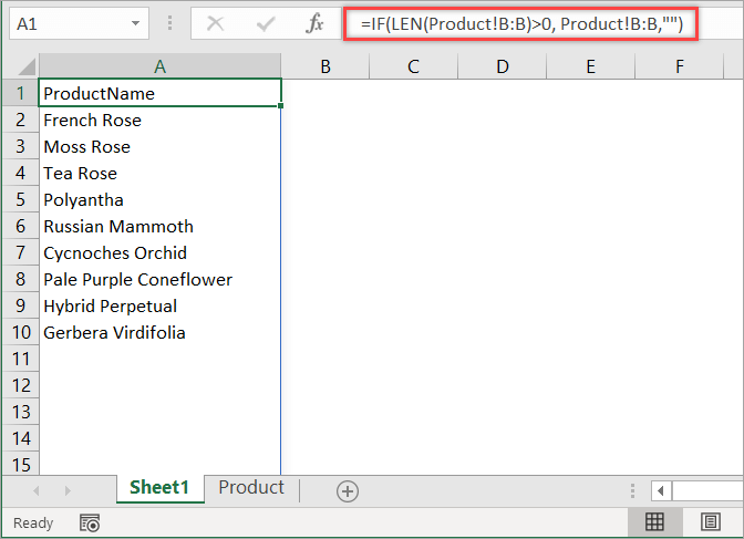
However, if you notice, the blank cells are showing zeros. If you want to see empty cells when there is nothing in the original sheet, you can change the formula to the one below:
=IF(LEN(Product!B:B)>0, Product!B:B,"")
How to link to a defined name in other sheets in Excel
For most people, words are easier to remember than numbers or codes. For this reason, Excel allows you to name an individual cell or range of cells. Then, you can use these names when referring to data in another sheet instead of typing the range address.
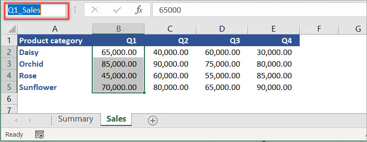
With the following worksheet, let’s create a defined name for the range B2:B5 and name it Q1_Sales.
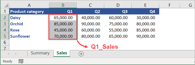
First, select the range of cells to include (B2:B5). Then, in the Name Box, type Q1_Sales and press Enter — and Done!
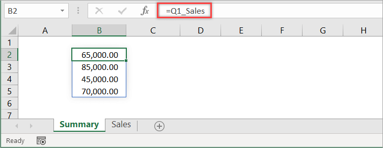
By default, Excel creates the name at the workbook level. To reference the defined name in another worksheet, just type the following formula into any cell.
=Q1_Sales
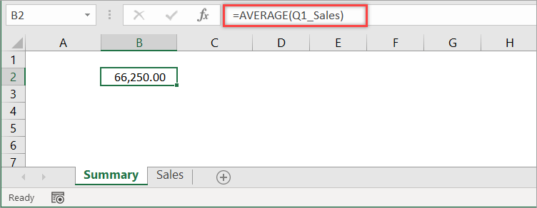
You can also use the defined name with an Excel function in a formula. For example, the following formula calculates the average of Q1_Sales:
=AVERAGE(Q1_Sales)
How to link lists in different sheets in Excel
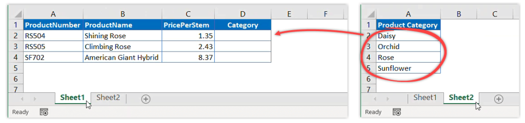
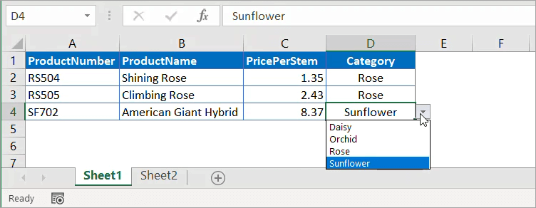
With the following spreadsheet, suppose you want to create a dropdown list in Sheet1 that contains product category data from Sheet2. This will allow you to select the Category in Column D using a dropdown instead of typing it manually.
Follow these steps:
- In Sheet1, select the range you want to apply to the dropdown list, which is D2:D4.
- Click Data > Data Validation.
- In the “Data Validation” dialog box, enter the following details, then click OK.
- Allow :
List - Source :
=Sheet2!$A$2:$A$5
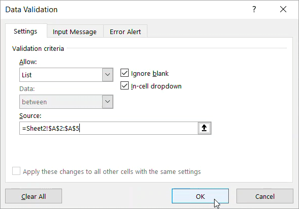
We enter a link reference to product category data in Sheet2, which is in range A2:A5. As a result, now you select the product category in Sheet1 using a dropdown, as shown below:
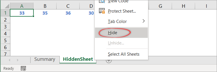
A sheet can be hidden for different reasons. For example, you may want to hide sheets that are no longer frequently being used by other users.
To create a link to a hidden sheet, simply unhide it first, create the link, and then hide it again if necessary.
You can actually refer to hidden sheets without unhiding them first, as long as you know the name of the sheets and the range you want to link from these sheets. However, most of the time, you’ll need to unhide them first to see the data you want to link so that you don’t accidentally refer to the wrong range of cells when creating the links.
There are two different types of hidden sheets in Excel: hidden and very hidden. While unhiding a hidden sheet is very easy, you will need to open the Visual Basic Editor (VBE) to unhide a very hidden sheet.
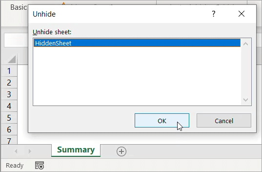
To link to a hidden sheet in Excel
- Unhide the sheet by right-clicking on any visible sheet, then select Unhide.

- In the “Unhide” dialog box that appears, select the sheet you want to unhide, then click OK.
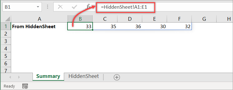
- Use a linking formula to link the data you want to show in another sheet.
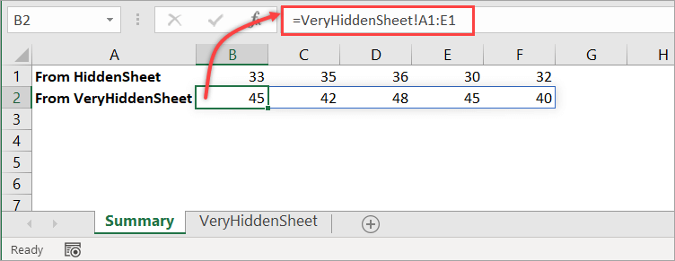
For example, the following formula in the Summary sheet shows the range A1:E1 from the sheet we just made visible.
=HiddenSheet!A1:E1
- If you want, hide the sheet again by clicking on the sheet tab, then select Hide.
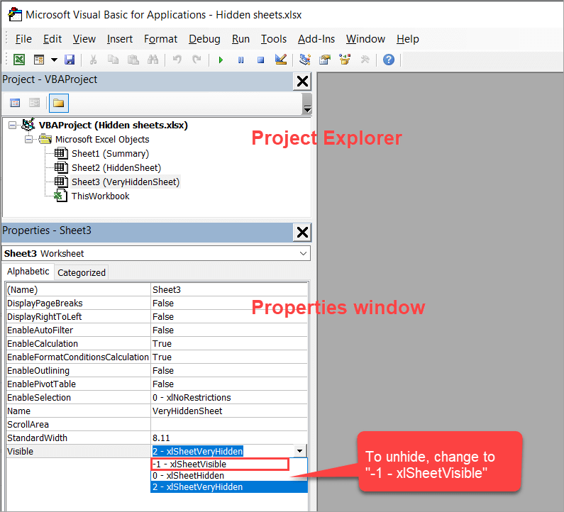
To link to a very hidden sheet in Excel
- Open the VBE by pressing Alt+F11.
- Press F4 or click View > Properties Window to open the Properties window under the Project Explorer if it’s not already open.
- In Project Explorer, select the very hidden sheet you want to unhide. Then, set its Visible property to
-1 - xlSheetVisiblein the Properties window.
- Use a linking formula to link the data you want to show in another sheet. For example, the following formula in the Summary sheet shows the range A1:E1 from the very hidden sheet we just made visible.
=VeryHiddenSheet!A1:E1
- If you want, change the sheet’s Visible property back to
2 - xlSheetVeryHiddenin the Properties window to make it a very hidden sheet again.
How to link sheets in Excel to a master sheet
With the following spreadsheet, suppose you want to link data from two worksheets into one.
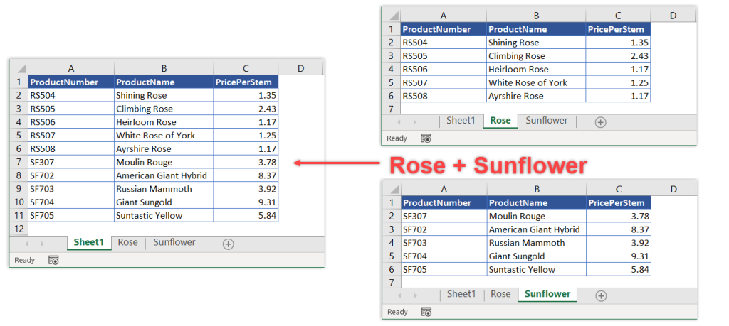
Notice that it’s like combining two ranges, which are Rose!A1:C6 and Sunflower!A1:C6.
However, combining ranges in Excel using a formula is a bit complex. An easier way to do this is using Power Query, as explained in the steps below:
- In the Rose sheet, select the range A1:C6.
- Then, on the Data tab in the Get & Transform Data section, click From Table/Range.
- In the “Create Table” dialog box, ensure that the My table has headers option checked.
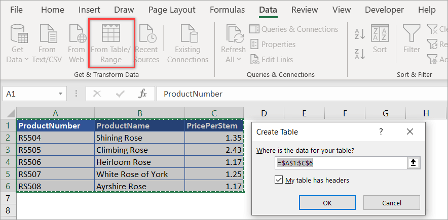
- Click OK — this will bring you to the Power Query editor.
- In the Query Settings, give your query a descriptive name, e.g., Roses.
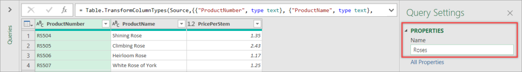
- Click the Home tab, then click Close & Load > Close & Load To…
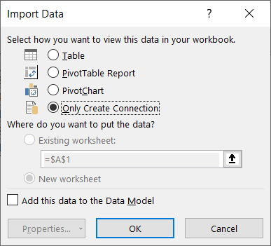
- In the “Import Data” dialog box, select Only Create Connection, then press OK.
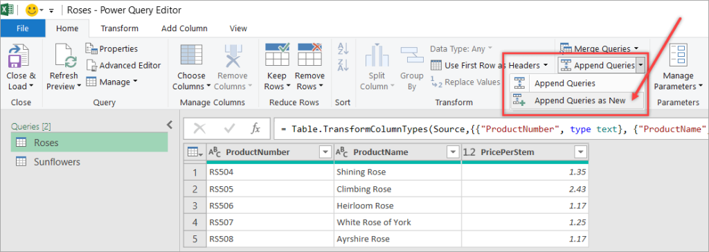
- Repeat steps 1-7 for the Sunflower data. But for the fifth step, let’s rename the query as Sunflowers.
- Re-launch the Power Query editor by clicking the Data tab, then click Get Data > Launch Power Query Editor…
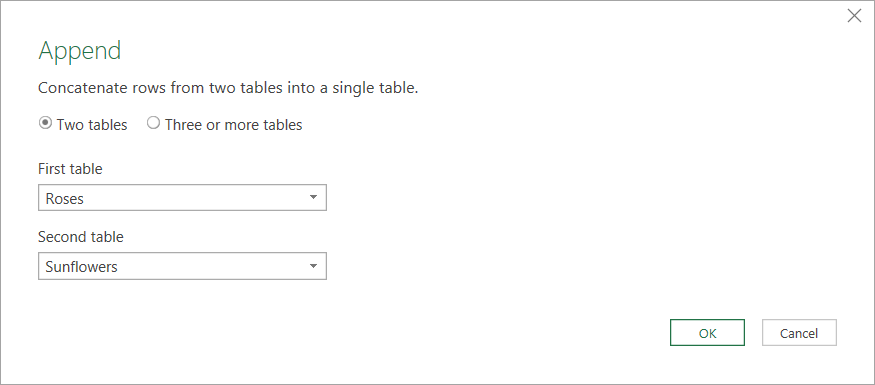
- Select any query, then click Append Queries > Append Queries as New to keep the existing queries unchanged.
- In the Append window, select the other table as the second table, then click OK.
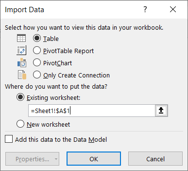
- Make sure to select the newly created query. Then, on the Home tab, click Close & Load > Close & Load To…
- In the “Import Data” dialog box, load the combined data to Sheet1!A1, then click OK.
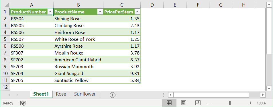
To see the result, click Sheet1. You’ll find the combined data as shown in the following screenshot:
When the source data from the other sheets changes, you won’t see the new changes right away. Using this method, you need to click the Refresh All button in the Data tab to see the latest data.
How to link two Excel sheets in different workbooks
To link to a worksheet in another workbook, you can do it whether the source file is open or closed. If possible, we suggest you open all the source workbooks first before creating the links in the destination workbook. Why? Because this way is easier.
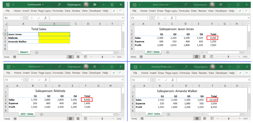
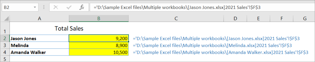
As an example, suppose you have the following four workbooks: Summary.xlsx, Jason Jones.xlsx, Melinda.xlsx, and Amanda Walker.xlsx. In the Summary workbook, you want to link the total sales of each salesperson, which is in cell F3 of each of the other workbooks—see the following screenshot:
Link to another worksheet when the source workbook is open
When all the source files are open, you can follow the steps below to create the links:
- In the Summary workbook, type = (equal sign) in the destination cell for Jason Jones.
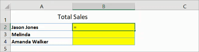
- Click View > Switch Windows, then select Jason Jones.xlsx to switch to this workbook.
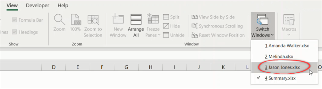
- Select the cell to link, in this case, F3, then press Enter.
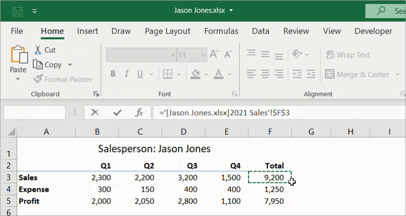
- Repeat Steps 1-3 for Melinda and Amanda Walker.
As the final result, you’ll see formulas with the following format when you click on each of the destination cells:
='[SourceWorkbook.xlsx]SheetName'!RangeAddress
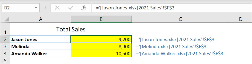
Note: In the above example, the workbook name and/or sheet name contain spaces, so the path is enclosed in single quotation marks.
Link to another worksheet when the source workbook is closed
If you close the source workbooks one by one, the linking formulas in the Summary workbook will change as shown in the below screenshot:
Now, you get the idea — you need to use the full path when linking to a workbook that’s currently closed.
Basically, you can use the following format to link data from any Excel workbook:
='FolderPath\[SourceWorkbook.xlsx]SheetName'!RangeAddress
However, if possible, just open the source files before you create the link, so you don’t need to manually type the long formula that’s shown above. ?
Can you break links between sheets in different workbooks in Excel?
When you open an Excel file, there may be formulas in it that get data from another workbook.
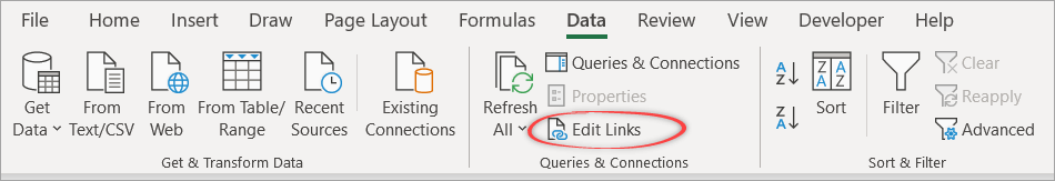
To locate these formulas, click on the Data tab in the ribbon. If the Edit Links button is available, it means that your file contains links to other workbooks.
To break a link, follow these steps:
- On the Data tab, in the Queries & Connections section, click Edit Links.
- In the “Edit Links” dialog box that appears, select the link you want to break and click Break Link.
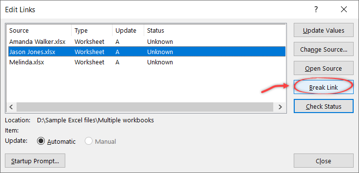
- Click Break Links in the confirmation dialog box that appears.

Notice that when you break a link to the source workbook, all the linking formulas are converted to their current values. This action cannot be undone, so you may want to back up your workbook before breaking any links.
- Click Close.
In this section, you’ve learned the basics of how to link sheets from different workbooks, as well as how to break those links. If you’re interested in more examples of linking worksheets from different workbooks, check out our article on how to link Excel files.
Why link data between sheets in Excel?
Linking sheets in Excel can be a great way to organize your data and keep them consistent across different worksheets. You may want to do this for different purposes, for example:
- You have a workbook containing data split by month, by state, or by salesperson, and you want a summary in one of the sheets.
- You want to create lists using links from different sheets in Excel.
- You want to collect data from multiple sheets and combine them into one to create a master sheet. Or, you may want to link data from a master sheet so that your data in other sheets are always up-to-date.
- Your data is growing and becoming too voluminous. As a result, you split it into different workbooks to be managed by different people. There can be times when you need to write formulas to get data out of these files.
Creating links between sheets is pretty easy to do. Besides, the main benefit is that whenever your data in the source sheet changes, the data in the destination sheet will be automatically updated as well.

Automate data export with Coupler.io
Get started for free