Let’s assume you’ve stumbled upon a useful table on some website and want to scrape this useful tabular data into your spreadsheet for analysis. You may try to copy and paste it manually, but that’s a layman’s way. Google Sheets has a handy function, IMPORTHTML, to do the job. It will import the table easily and refresh your data at regular intervals to keep it updated.
In this article, you’ll learn how to use the IMPORTHTML function to fetch tables and lists from a web page easily.
How does the IMPORTHTML function work in Google Sheets?
The Google Sheets IMPORTHTML function looks for a specific HTML table or list and copies the data out of it. You can use it to scrape texts within a table or list. An HTML table is defined by the <table> tag, while a list is defined by the <ul> (for unordered list) and <ol> (for ordered list) tags.
How to use IMPORTHTML formula in Google Sheets
Before using the IMPORTHTML formula, let’s understand its syntax.
=IMPORTHTML(URL, query_type, index)URL— The URL of the page, including protocol (http://orhttps://). Make sure to enclose the URL within double-quotes.query_type— Use “table” if you want to import a table, otherwise “list” if you’re going to import a list.index— The index of the table or list on the web page. It starts at 1. A table with index =1means that it’s the first table, index =2means that it’s the second table, and so on.
Import website data to Google Sheets with IMPORTHTML
How to get indexes of tables/lists to pull data from a website to Google Sheets using IMPORTHTML
A page may contain one or more tables and/or lists. If you have no idea how to find the indexes of tables on an HTML page, follow the steps below:
Step 1
Open your browser’s Developer console. For most browsers on Windows, you can open the console by pressing F12. If you’re using a Mac, use Cmd+Opt+J for Chrome, and Cmd+Opt+C for Safari. Note that, for Safari, you’ll need to enable the “Develop menu” first.
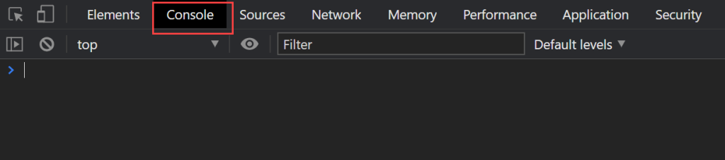
The exact look will depend on the version of Google Chrome you’re using. It may change from time to time, but should be similar.
Step 2
Copy and paste the following code into the console to get indexes of all tables:
var index = 1; [].forEach.call(document.getElementsByTagName("table"), function(elements) { console.log("Index: " + index++, elements); });
If you are looking for all lists’ indexes instead, you need to get all elements with tag <ul> or <ol>. The following code may help you:
var index = 1; [].forEach.call(document.querySelectorAll("ul,ol"), function(elements) { console.log("Index: " + index++, elements); });
Step 3
Press Enter. You will see numbers that represent indexes shown in the results. Move your cursor over the elements in the result until the table/list you want to display is highlighted.
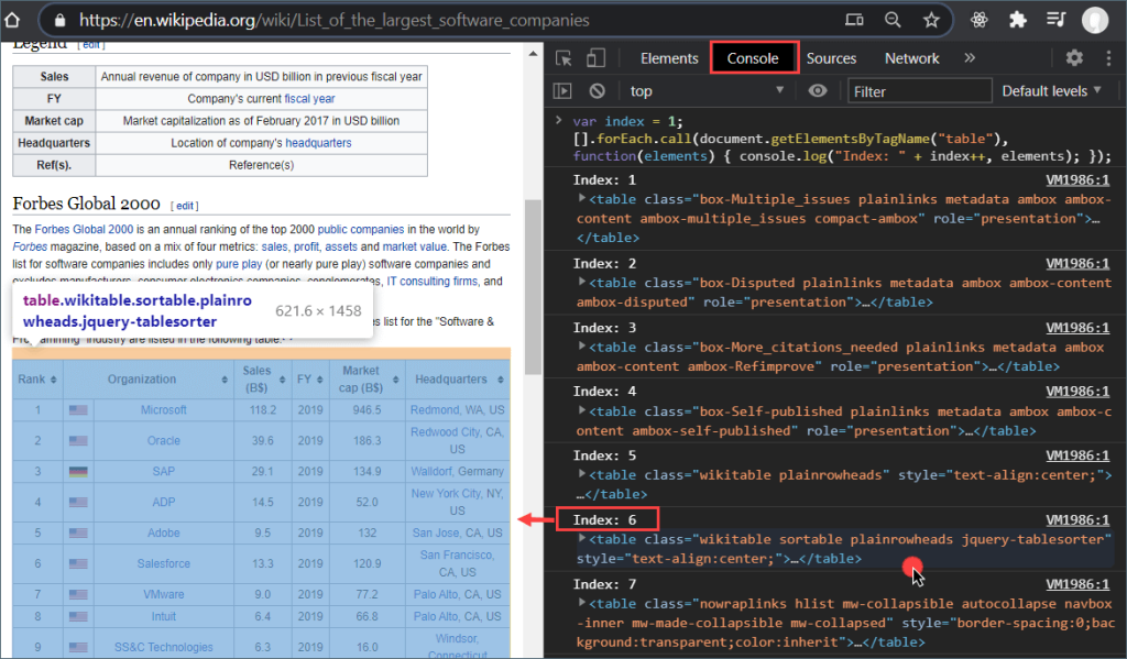
As you can see in the screenshot above, the table highlighted has index = 6.
How to import an HTML table into Google Sheets
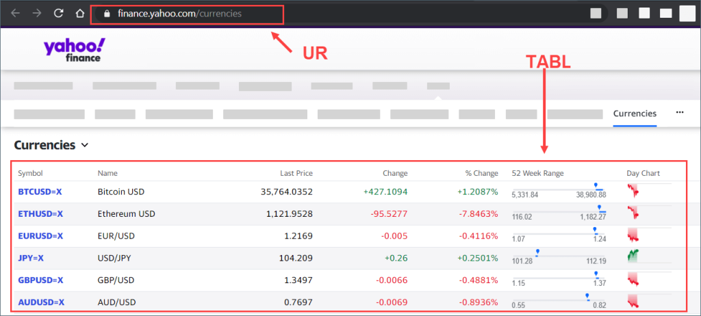
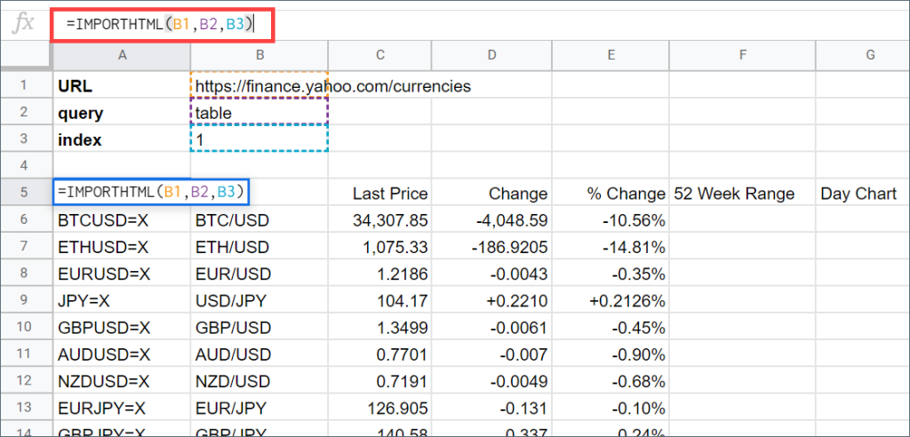
Let’s see how we can import an HTML table. We will pull the latest currency exchange rates data from Yahoo! Finance Currencies website to Google Sheets. The page only has one table, so we’ll use 1 for the index value.
Now, create a new blank Google spreadsheet and give it a name – for example, Currencies. Then, copy and paste the following formula into A1.
=IMPORTHTML("https://finance.yahoo.com/currencies","table",1)
Then, press Enter and wait until the entire table is populated in the spreadsheet.
In the above image, we can see that the IMPORTHTML function successfully grabbed the latest currency rate data into Google Sheets.
You may be interested in monitoring the exchange rate data. In that case, you may want to check our tutorial on how to build a currency exchange rate tracker in Google Sheets without coding.
How to import a list into Google Sheets
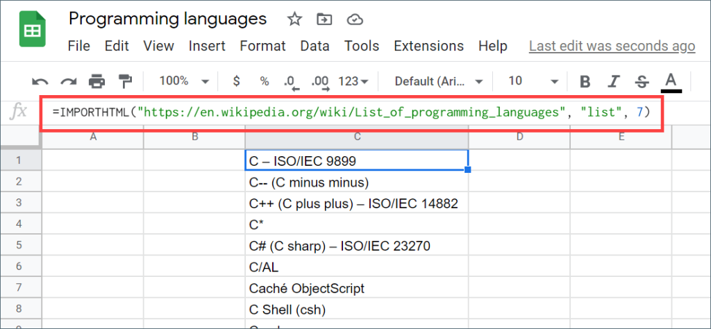
You can import a list using the same method. The only change would be to replace the word “table” with “list” in the parameter. The following steps demonstrate how to pull data from a list containing programming languages starting with the letter “C“.
Create a new blank Google spreadsheet and give it a name. Then, copy and paste the following formula into C1:
=IMPORTHTML("https://en.wikipedia.org/wiki/List_of_programming_languages","list",7)
Press Enter and wait for the data to populate, as the following screenshot shows:
Other options for scraping data into Google Sheets
Use Google Sheets functions
If you’re looking for another method to retrieve data from different structures besides HTML tables and lists, here are some Google Sheets functions you may want to try:
| Function name | Description |
|---|---|
IMPORTXML | This function imports data from various structured data types including XML, HTML, CSV, TSV, as well as RSS and ATOM XML feeds. |
IMPORTRANGE | This function imports a range of cells from a specified spreadsheet. |
IMPORTFEED | This function imports an RSS or ATOM feed. |
IMPORTDATA | This function imports data in CSV or TSV format from a URL. |
Import data from cloud sources with Coupler.io
If you want to import data from other sources and apps or load data via APIs without coding, you can use Coupler.io. This reporting automation platform can extract data from over 60 various sources and transfer it to Google Sheets automatically on a schedule.
The supported data sources include:
- Financial apps – Xero, QuickBooks, Stripe, etc.
- CRMs – Pipedrive, HubSpot, Salesforce, etc.
- Data warehouses – MySQL, BigQuery, Redshift, PostgreSQL, etc.
- Ecommerce – Shopify, WooCommerce, etc.
- Sales apps – Pipedrive, Calendly, Google Calendar, etc.
- Marketing apps – GA4, Google Ads, LinkedIn Ads, and many others.
Additionally, Coupler.io offers a JSON integration to scrape data via APIs into Google Sheets without writing a single string of code. On top of that, it allows you to channel data from Google Sheets to dozens of other applications. Let’s see how it works.
Select your data source in the form below and click Proceed.
In order to use the platform, you will be required to create a Coupler.io account (it’s free, no credit card is required). Then, follow the onscreen instructions to connect your data source account.
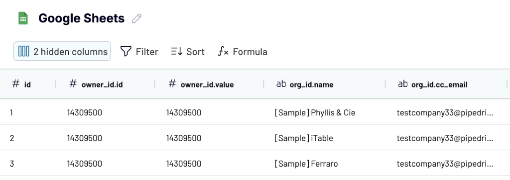
In the next step, preview your data and transform it, if needed. For example, you can rearrange and rename columns, hide the columns you don’t need or add new calculated columns, sort and filter data, and more.
In addition, Coupler.io allows you to merge data from several sources into a single dataset (based on column names).
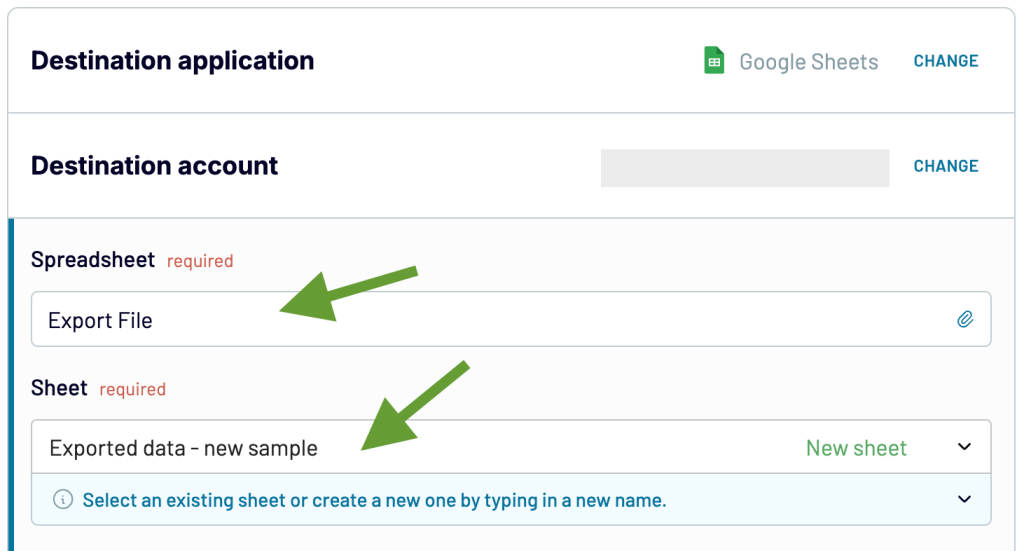
Then, connect your Google account to extract data from. Specify the spreadsheet and the sheet where to load your data.
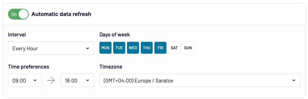
Once this is done, set up your custom schedule for data refreshes. Depending on your needs, Coupler.io can extract the latest information from your selected data source and send it to Google Sheets as often as every 15 minutes.
Finally, save and run the importer to transfer your data. Your auto-updating report is ready.
How to reference a cell in IMPORTHTML in Google Sheets
You may want to put the URL and other parameters in cells, then refer to them when using the IMPORTHTML formula. In this case, you can change the parameters more easily by editing the cell values.
Here’s an example:
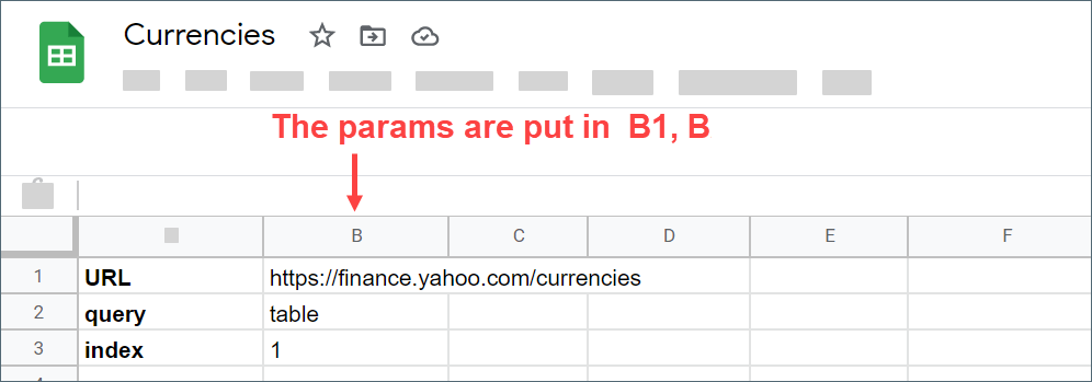
All params for URL, query, and index are put in B1, B2, and B3. Thus, you can easily write the IMPORTHTML formula as follows:
=IMPORTHTML(B1,B2,B3)
Let’s look at another example. Suppose you want to get the latest historical rates of the EUR/USD currency pair from this page:
https://finance.yahoo.com/quote/EURUSD%3DX/history?p=EURUSD%3DXYou can put the string EURUSD in a cell – for example, B1. In this case, if you want to fetch other currency data, you’ll just need to change the value in B1. Here’s an example of how to refer to the B1 cell in the Google Sheets IMPORTHTML formula:
=IMPORTHTML("https://finance.yahoo.com/quote/" & B1 & "%3DX/history?p=" & B1 & "%3DX", "table", 1)
Now, let’s add the above formula into A3:
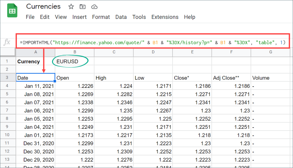
If you want to pull historical data for AUD/USD, change B1‘s value to AUDUSD, and your data will refresh automatically.
Tip: You can avoid typing B1 multiple times by using the SUBSTITUTE function. Here’s what the updated formula looks like:
=IMPORTHTML(SUBSTITUTE("https://finance.yahoo.com/quote/{{CURRENCY}}%3DX/history?p={{CURRENCY}}%3DX", "{{CURRENCY}}", B1), "table", 1)
How to use IMPORTHTML to import a portion of a range table data to Google Sheets
Want to pull just a few columns? Or filter only rows with specific criteria? You can achieve these things by using the QUERY function in combination with IMPORTHTML.
IMPORTHTML: Importing specific columns
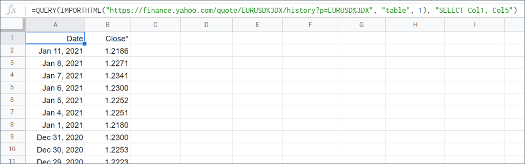
Suppose you have a sheet with an IMPORTHTML function that pulls the latest EUR/USD rate data from a website to Google Sheets.
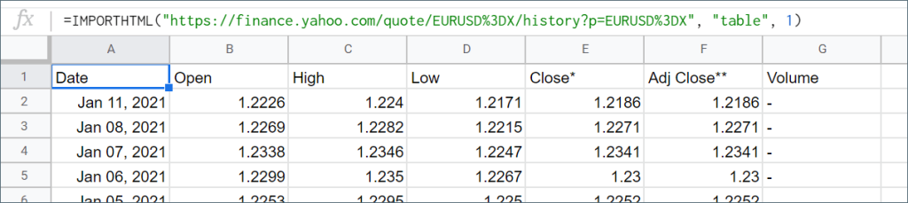
Now, you only want to retrieve the Date and Close columns that are the 1st and 5th columns. To do that, you can combine your existing formula with the QUERY function — here’s an example:
=QUERY(IMPORTHTML("https://finance.yahoo.com/quote/EURUSD%3DX/history?p=EURUSD%3DX", "table", 1), "SELECT Col1, Col5")
By defining “SELECT Col1, Col5” in the QUERY function, you will get this result:
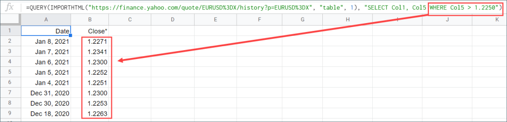
IMPORTHTML: Importing specific rows
You can also retrieve specific rows. For example, here’s how to add a filter to our previous formula to fetch just the data with Close values higher than 1.2250:
=QUERY(IMPORTHTML("https://finance.yahoo.com/quote/EURUSD%3DX/history?p=EURUSD%3DX", "table", 1), "SELECT Col1, Col5 WHERE Col5 > 1.2250")
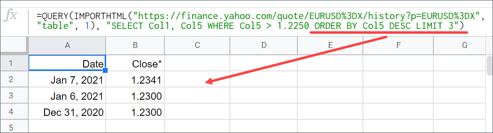
Now, let’s add one more filter to fetch just the top 3 highest rates. Here’s the formula:
=QUERY(IMPORTHTML("https://finance.yahoo.com/quote/EURUSD%3DX/history?p=EURUSD%3DX", "table", 1), "SELECT Col1, Col5 WHERE Col5 > 1.2250 ORDER BY Col5 DESC LIMIT 3")
How to set a custom interval to automatically refresh IMPORTHTML in Google Sheets
By default, the Google Sheets IMPORTHTML refresh period is every 1 hour. However, you can speed up the refresh interval if you want. As the formula is recalculated when its arguments change, you can use this to force the refresh interval. The idea is to concatenate the original URL with a query string that changes periodically based on the time we set – for example, every 5 minutes. Here are the steps:
First, add a query string in the original URL
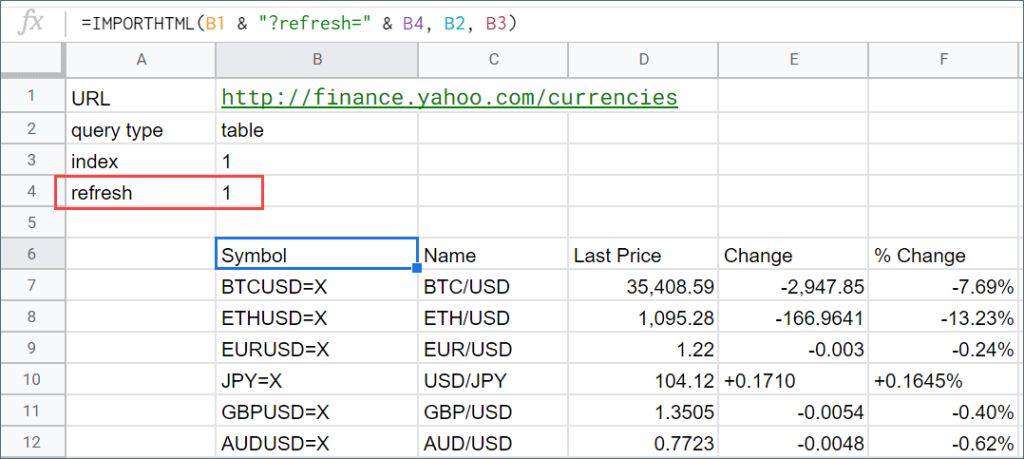
Suppose we have the following values in B1-B5. The IMPORTHTML function is defined in B5. Notice that a query string "?refresh=" & B4 is added to the original URL.
| Note | Cell | Value |
| URL | B1 | https://finance.yahoo.com/currencies |
| query type | B2 | table |
| index | B3 | 1 |
| refresh | B4 | 1 |
| formula | B5 | =IMPORTHTML(B1 & "?refresh=" & B4, B2, B3) |
The sheet looks as follows:
We’re not done yet. Let’s continue to the next step.
Next, use script and trigger to automate refresh
We are going to refresh the value of B4 every 5 minutes using a script and trigger. As a result, the Google Sheets IMPORTHTML formula will also refresh at the same interval. Follow these instructions:
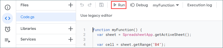
Step 1. Go to the Script editor (either Tools > Script Editor or Extensions > App Script).
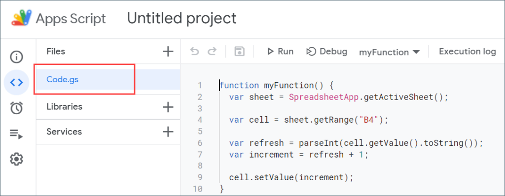
Step 2. Copy and paste the following code in the Code.gs. Then, save your changes by pressing the Disk icon in the toolbar.
function myFunction() {
  var sheet = SpreadsheetApp.getActiveSheet();

  var cell = sheet.getRange("B4");

  var refresh = parseInt(cell.getValue().toString());
  var increment = refresh + 1;

  cell.setValue(increment);
}
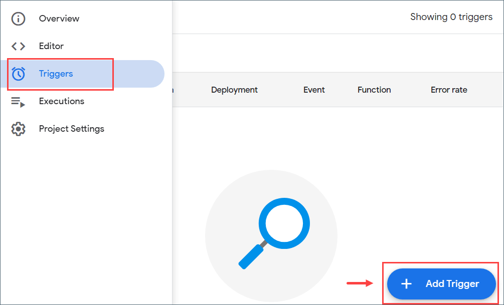
Step 3. Open the Triggers menu on the left, then click the Add Trigger button.
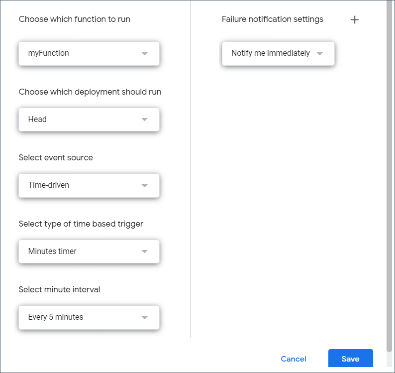
Step 4. Set a trigger for myFunction so that it runs every 5 minutes. Optionally, you can set the Failure notification settings to Notify me immediately so that you receive a notification immediately when an error occurs.
Step 5. Click the Save button. If you are asked to authorize the script to access your data, grant the permission.
Step 6. Run your script for the first time.
Now, you’ll be able to see the data on your sheet refresh every 5 minutes. Even when your Google Sheet is closed, it will continue to refresh.
How many IMPORTHTMLs can Google Sheets handle?
You can use the IMPORTHTML in a Google spreadsheet as many times as you want. Before, the limit was 50 per Google spreadsheet for external data, but Google removed this limitation in 2015. As Google Sheets is web-based, you may experience a drop in speed if you have lots of IMPORTHTML formulas in your spreadsheet especially if your internet connection is slow.
How to pull non-public data from a website into Google Sheets using IMPORTHTML function
You may want to pull data from a non-public URL on a website into Google Sheets. Unfortunately, you can’t do that using the IMPORTHTML function. See the following screenshot, which shows what happens if you try scraping your LinkedIn network list.
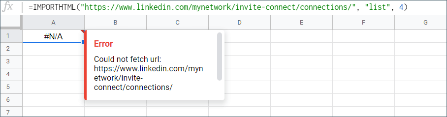
The formula only works if the page is publicly available and does not require you to log in to access the data. You’ll get an error message #N/A Could not fetch url for accessing non-public URLs.
To extract non-public data, we recommend you use Coupler.io. You will need to connect the app from which you want to get non-public data and then connect your Google account. This process takes just a couple of minutes. Coupler.io can regularly update the imported non-public data in your Google Sheets workbook according to your schedule.
What to do if the IMPORTHTML formula is suddenly not working in your Google Sheets
If your formula suddenly stops working, we recommend you do the following::
- Check for URL changes. Although it’s a rare case, it’s possible that the page you scrape has been moved to another URL.
- Check for protocol change. For example, the site you’re scraping is now using https instead of http, but the auto-redirect to https is not set up yet by the website owner.
- Check for index change. The table or list with index = 9 could have index = 8 now.
If you still can’t pull the data you want, then it could be that the website owner now blocks bots/crawlers from reading their web content. Check the website’s robots.txt by navigating through <website_url>/robots.txt.
Google Sheets IMPORTHTML Error Loading Data
This Error Loading Data is one of the most common issues with IMPORTHTML. You most likely face it trying to pull data from websites that use large scripts. They take a long time to run and hence can be risky in terms of security. This means that you can’t parse pages with JS using IMPORHTML to Google Sheets.
In this case, you can try to find just find a different source with the necessary data or opt for an alternative data importing option, for example via the API using the JSON importer by Coupler.io. Good luck!

Automate data import to Google Sheets with Coupler.io
Get started for free