Excel VLOOKUP is one of the most useful functions as it allows you to easily navigate your data and save significant time. It can be used to calculate totals and averages, update product prices, quickly look up customer information, and much more.
In this blog post, we explain how to VLOOKUP in Excel with two spreadsheets. In particular, you will learn how to use this function with two different workbooks, with two worksheets, and also how to VLOOKUP another Excel Online file. Let’s dive in!
How to VLOOKUP another workbook in Excel
Before we dive into the details of using the VLOOKUP function, we will need a sample dataset to work with, so this will be our step 1.
We imported a dataset from Google Sheets to Excel using Coupler.io, a solution that allows you to automatically transfer data from 70+ sources to Excel and other apps.
Read more about Microsoft Excel integrations for data export on a schedule.
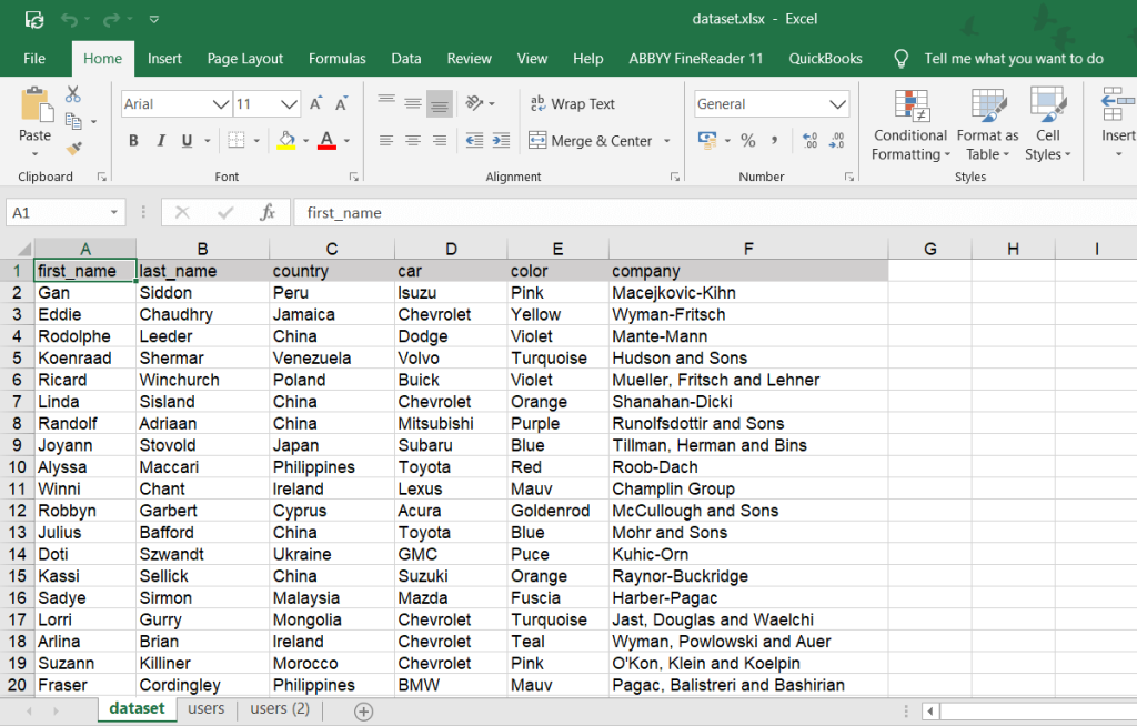
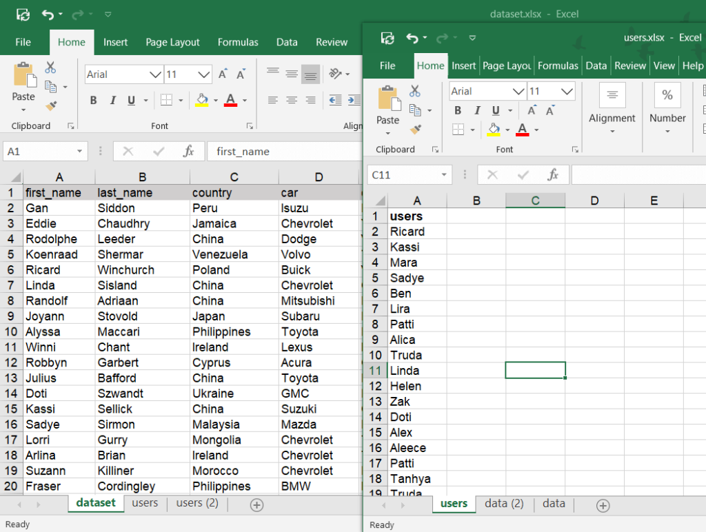
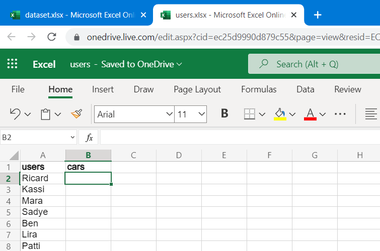
The data was imported to the workbook titled “dataset” – this is our lookup range. The lookup values are stored in another spreadsheet, titled “users“.
Now, let’s VLOOKUP these two spreadsheets.
How to VLOOKUP between two workbooks: step-by-step instructions
To VLOOKUP between two workbooks, complete the following steps:
- Type
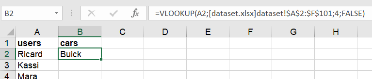
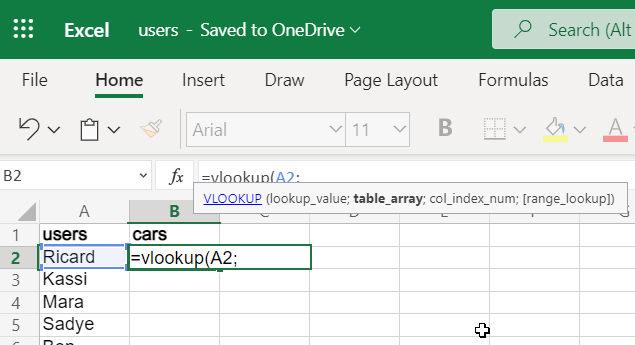
=vlookup(in the B2 cell of the users workbook.
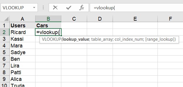
- Specify the lookup value. You can enter a string wrapped in quotes or reference a cell just like we did:

- Enter a comma/semicolon (depending on the list separator defined under your regional settings), click on the spreadsheet with the range you want to look up and select the desired range. In our case, the unfinished formula looks like this:
=vlookup(A2,[dataset.xlsx]dataset!$A$2:$F$101
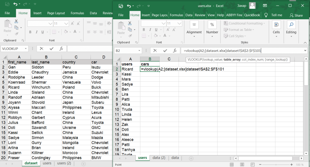
So, basically, you can manually type the range to lookup using the following sample:
[dataset.xlsx]dataset!$A$2:$F$101
[dataset.xlsx]– name of the spreadsheetdataset!– name of the worksheet$A$2:$F$101– locked range to lookup
- In the formula bar, add a comma/semicolon and enter the column number, which contains the matching value to return. In our case, the number is 4 (column D).
=vlookup(A2,[dataset.xlsx]dataset!$A$2:$F$101,4
- Add a comma/semicolon and enter FALSE to return the exact match. Close the bracket and hit enter
=vlookup(A2,[dataset.xlsx]dataset!$A$2:$F$101,4,FALSE)
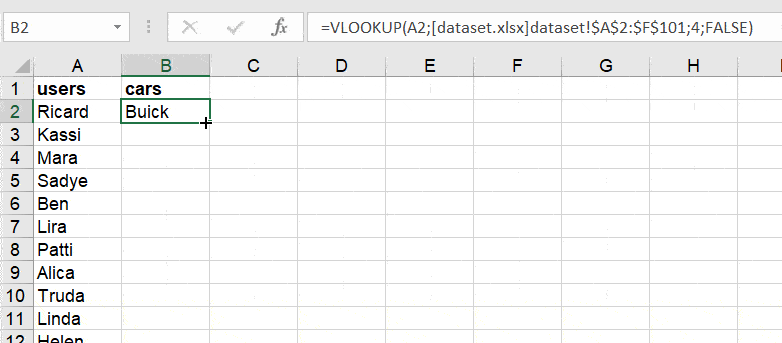
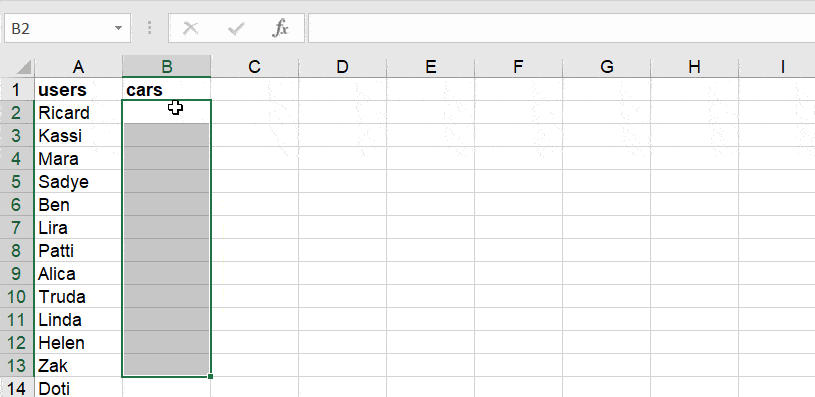
To return the matching values for other users, we can drag the formula down:
Or use an array formula:
- You need to specify an array as a lookup value
=VLOOKUP(A2:A66,[dataset.xlsx]dataset!$A$2:$F$101,4,FALSE)
- Then select an array where to return the matching values, insert the VLOOKUP formula into the formula bar and press Ctrl+Shift+Enter for Windows (Command+Return for Mac)
Now you know how to VLOOKUP between two workbooks. You can go through the same steps to VLOOKUP between multiple workbooks as well, not just two.
How to VLOOKUP between two worksheets
But what if your datasets are not located in different workbooks and you need to VLOOKUP between two worksheets? The process is exactly the same as for using VLOOKUP with two workbooks, which we already described in detail in the section above. The only difference is that you don’t need to include the workbook name in the formula, since both worksheets are a part of the same workbook.
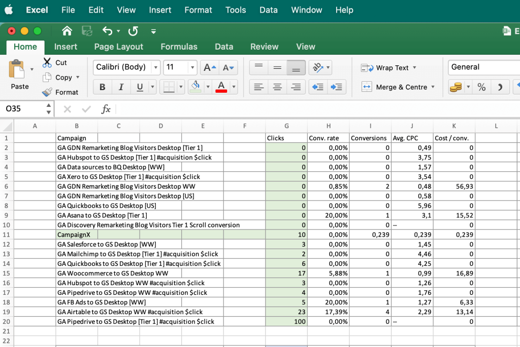
Let’s see how this works. In this example, we used Coupler.io to transfer data from Google Analytics to Excel. Now, we have two datasets on two different sheets in the same workbook. Let’s open the first dataset. On sheet 1, we have a list of ad campaigns, and we need to fetch the data about the number of clicks for each campaign. This information is located on sheet 2.
To extract the number of clicks, we can use the following formula:
=VLOOKUP(lookup_value, table_array, col_index_num, [range_lookup])
You already know the main elements:
lookup_value – what we are looking for; in our example, it will be CampaignX
table_array – where to look for the information; here, it’s Sheet2!B2:V20
col_index_num – the column index is the number of the column to return value from; here, it’s 12 – the “Clicks” column on Sheet 2
[range_lookup]– we select FALSE to get the exact match; you can also select TRUE for an approximate match
So, our ready-to-use formula looks like this:
=VLOOKUP(Sheet2!B11; Sheet2!B2:V20; 12; FALSE)
(You can also use commas instead of semicolons – just use the separator specified in your settings).
We insert/type it into the cell where we want to get the returned values and hit enter. Here’s the result:
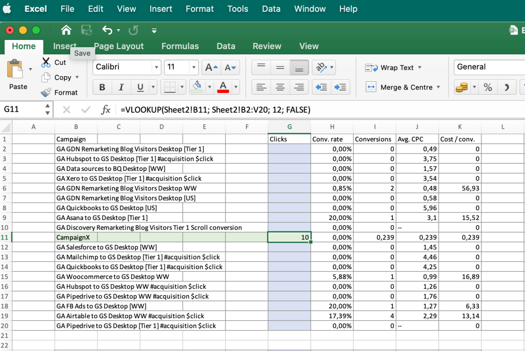
The formula searched for Campaign X on sheet2 and fetched the corresponding value from the specified column (in our example, column 12 – Clicks). The extracted value was then displayed on sheet1.
Then, we simply drag the formula to the other cells to return the number of clicks for all the campaigns listed in the second column. (For more details, see the GIF in the section above – dragging formulas works in the same way here).
Now, all the range of cells in the “Clicks” column is filled with the data fetched from the second sheet.
As you see, it’s pretty easy to VLOOKUP between two worksheets, especially if you are comfortable with using Excel formulas. But, of course, you can use the same formula to VLOOKUP between multiple sheets, not just two. Hope this helps!
How to VLOOKUP another Excel Online file
Unfortunately, the flow described above for VLOOKUP does not work with Excel Online workbooks. You can’t select the range to look up from another spreadsheet. The simplest way to solve this is to import the required data from another workbook (Excel to Excel) using Coupler.io and perform the vlookup as above.
Or you can look up from another spreadsheet using this syntax:
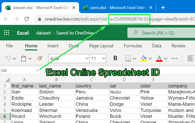
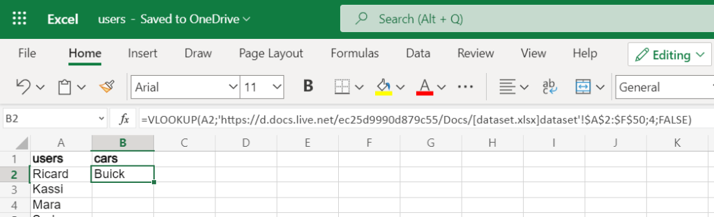
=VLOOKUP("lookup_value",'https://d.docs.live.net/spreadsheet-id/Docs/[spreadsheet-name.xlsx]sheet-name'!locked-lookup-range,column_number,match)Let’s see how it works in the example. We’ll use the same workbooks from above – dataset and users – but edited in Excel Online.
The parameters we need for our VLOOKUP formula are:
"lookup_value"– A2
- You can find the spreadsheet-id of your Excel Online workbook in the URL bar.
- The spreadsheet name and the range should not cause any trouble. But do not forget to lock the lookup_range using $ symbols. Now the VLOOKUP formula looks like this:
=vlookup(A2,'https://d.docs.live.net/ec25d9990d879c55/Docs/[dataset.xlsx]dataset'!$A$2:$F$50,column_number,match)
- As the last step, specify the column number and the match parameters. Now we can run our VLOOKUP formula:
=vlookup(A2,'https://d.docs.live.net/ec25d9990d879c55/Docs/[dataset.xlsx]dataset'!$A$2:$F$50,4,false)
With this syntax, you can either drag your VLOOKUP formula or apply an array formula as we described above.
That’s it! Just one more tip before you go. We all love Excel formulas because they allow us to automate tasks and save time. But using formulas is not the only way to do so. We recommend you try out a data automation solution as well – it allows you to automate even more data tasks and save a lot more time. Try Coupler.io’s Excel integrations with an online app or Excel add-on that works directly in a spreadsheet.
We hope our tutorial will help you to confidently VLOOKUP in Excel with two spreadsheets, be it two different workbooks, worksheets, or even Online Excel files. Or, in fact, you can VLOOKUP between any number of Excel sheets or files. Many thanks for reading!