Are you an experienced Google Sheets user? Then you probably know the options in Google Sheets to reference another sheet and use the IMPORTRANGE function for that. Meanwhile, you could become an expert and do better. Professionals combine IMPORTRANGE with QUERY and manipulate the imported dataset at the same time. If you want to join the experts and improve your Google Sheets skills – welcome to this blog post.
If you prefer watching to reading, check out our guide to QUERY & IMPORTRANGE in Google Sheets on the Coupler.io Academy YouTube channel.
IMPORTRANGE function explained
The IMPORTRANGE function allows you to import a data range from a specified spreadsheet.
IMPORTRANGE syntax
=IMPORTRANGE("spreadsheet_url","range_string")
spreadsheet_url– insert the URL of the spreadsheet to import data from. For example,
https://docs.google.com/spreadsheets/d/1h3pPtbMAsPM_jS2wMLG_GflqyAd
Alternatively, you can use the spreadsheet ID instead of the entire URL
1h3pPtbMAsPM_jS2wMLG_GflqyAd
range_string– insert a string that specifies the data range for the import. For example,Sheet1!A1:C13. The string consists of thesheet_name!and therange.range– specify the range of cells to import.sheet_name!– specify this parameter if you are not importing data from the first sheet of the document.
IMPORTRANGE formula example
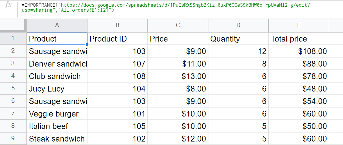
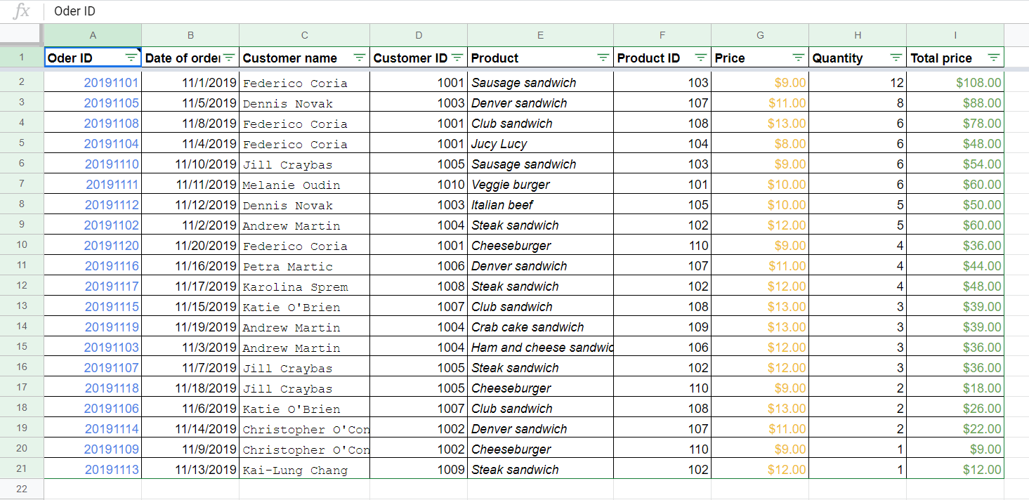
We have a database in the spreadsheet called Orders from Airtable. Let’s import all the values in the columns E to I. Here is the formula for this:
=IMPORTRANGE("https://docs.google.com/spreadsheets/d/1PuEsRXSShgbBKiz-6uxP6OGeS9kBHW0d-rpUAaMl2_g/edit?usp=sharing","All orders!E1:I21")
You can check out the formula example in this tab.

QUERY function explained
The QUERY function lets you manipulate data while importing it from another sheet. You can select, filter, sort, and do other manipulations.
QUERY syntax
=QUERY(data_range,"query_string")
data_range– insert a range of cells to query.data_rangemay include columns with boolean, numeric, or string values. If a column contains different data types, QUERY will pick the majority data type as the column data type.
query_string– insert a string made using clauses of the Google API Query Language. Alternatively, you can refer to a cell that contains thequery_string(in this case, avoid double quotation marks both in the QUERY formula and thequery_string).
Optionally, you can enhance the QUERY formula with a part that defines the number of headers in your data range. In this case, the QUERY syntax will be the following:
=QUERY(data_range,"query_string",headers_number)
One header row is used by default.
QUERY formula example
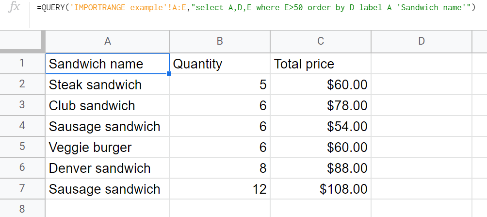
Let’s use the data range that we imported using IMPORTRANGE in the previous example and do the following manipulations:
- Select columns A, D and E.
- Filter out the products with a total price of more than $50.
- Order the outcome by quantity in ascending order.
- Change the A column header from “Product” to “Sandwich name”.
Here is the QUERY formula to do that:
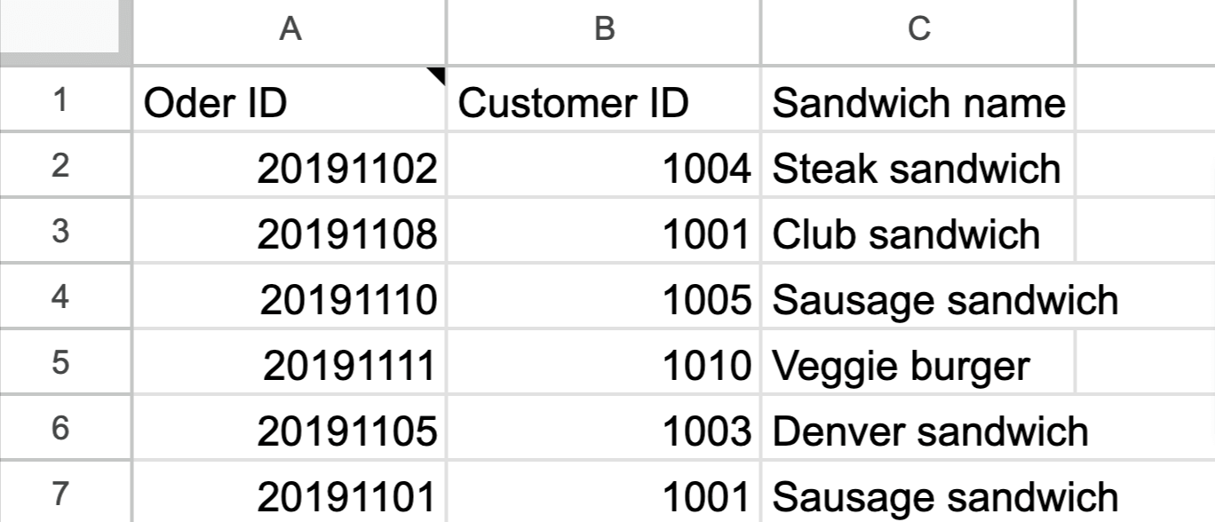
=QUERY('IMPORTRANGE example'!A:E,"select A,D,E where E>50 order by D label A 'Sandwich name'")
You can check out the formula example in this tab.
Though QUERY is a powerful function, it has a drawback: it only works within a spreadsheet. So, you can grab data from one sheet to another, but you can’t query another spreadsheet. The combination of QUERY+IMPORTRANGE is meant to handle this issue.
We blogged about this function in “Google Sheets Query”
How to combine QUERY and IMPORTRANGE in Google Sheets
When you apply QUERY and IMPORTRANGE together, you can query a data range in another spreadsheet (or multiple spreadsheets).
If you need a quick insight into using QUERY+IMPORTRANGE, check out this part of the IMPORTRANGE video tutorial by Railsware Product Academy. The needed timestamp is already setup:)
QUERY+IMPORTRANGE syntax
=QUERY(IMPORTRANGE("spreadsheet_url", "data_range"), "query_string")
spreadsheet_url– insert the URL of the spreadsheet to import data from.data_range– insert a range of cells to query.query_string– insert a string made using clauses of the Google API Query Language.
Optionally, you can enhance the formula with a part that defines the number of headers in your data range. In this case, the syntax will be the following:
=QUERY(IMPORTRANGE("spreadsheet_url", "data_range"), "query_string", [headers])
One header row is used by default.
QUERY+IMPORTRANGE formula example
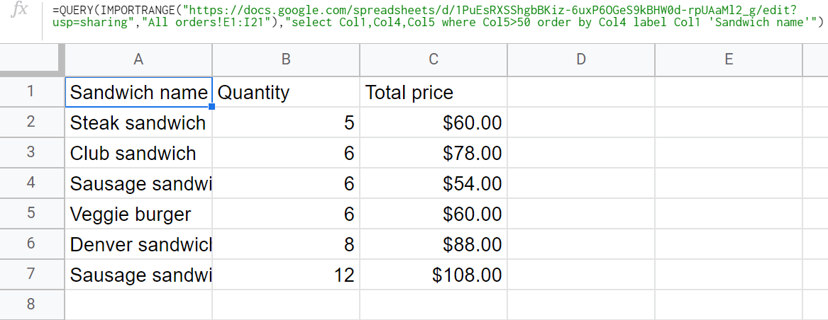
Let’s repeat the examples above but using only one formula. So, we need to:
- import a data set from the spreadsheet called Orders from Airtable.
- do a few manipulations with it:
- Select columns A, D and E.
- Filter out the products with a total price of more than $50.
- Order the outcome by quantity in ascending order
- Change the A column header from “Product” to “Sandwich name”.
Here is the formula:
=QUERY(IMPORTRANGE("https://docs.google.com/spreadsheets/d/1PuEsRXSShgbBKiz-6uxP6OGeS9kBHW0d-rpUAaMl2_g/edit?usp=sharing","All orders!E1:I21"),
  "select Col1,Col4,Col5 where Col5>50 order by Col4 label Col1 'Sandwich name'")
All orders!E1:I21 is our target data_range. During the import, the column reference will change as follows:
E to A, or simply Column #1 – Col1
F to B, or simply Column #2 – Col2
G to C, or simply Column #3 – Col3
H to D, or simply Column #4 – Col4
I to E, or simply Column #5 – Col5
That’s why we recommend you apply Col reference in your QUERY formulas to avoid errors.
You can check out the formula example in this tab.
How to query data from other spreadsheets without formulas
Using complex QUERY and IMPORTRANGE formulas can take too much time, not to mention potential syntax errors, combined with hiccups on Google’s end.
Fortunately, there’s an alternative solution. You can query your data range from other spreadsheets or even external data sources without any complex formulas with Coupler.io. What’s more, it enables you to automate data import from several spreadsheets to a single document.
This way, you can save hours of your time per month, avoid potential errors, and have your data constantly updated.
Use the form below to check this out. We’ve preselected Google Sheets as a source, but you’re free to select your option. Click Proceed and sign up with your Google account for free.
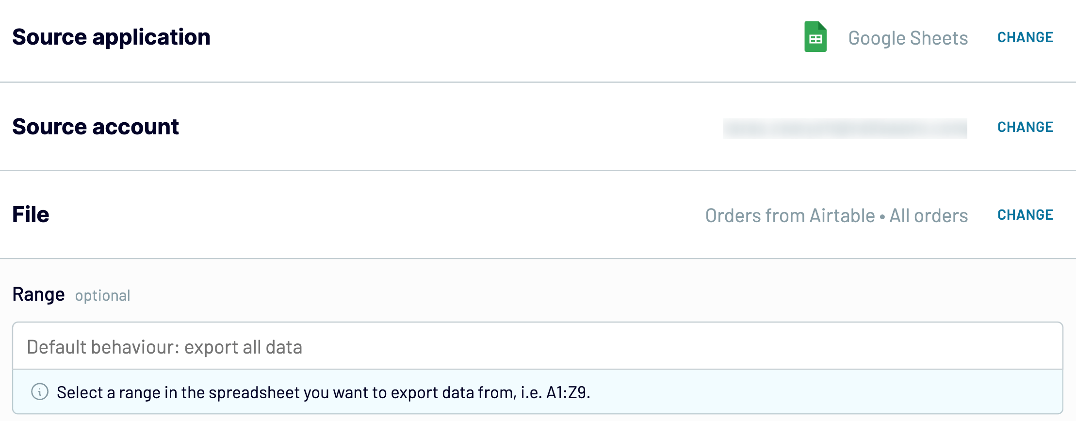
Let’s see how you can query data from the spreadsheet called Orders from Airtable just like we did in the example above.
Choose Orders from Airtable as the source file. Then specify your sheet – All orders – for data transferring. Optionally, you can select a particular range you’d like to export.
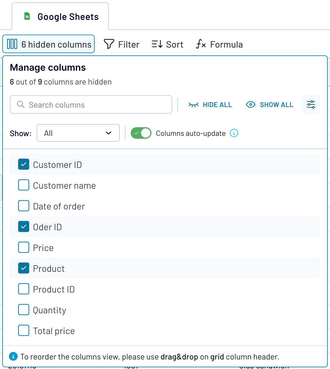
Proceed to the next step, where you can transform or query your data. Click Column Management and untick the columns except A, D, and E. This way, you hide unnecessary columns on the go.
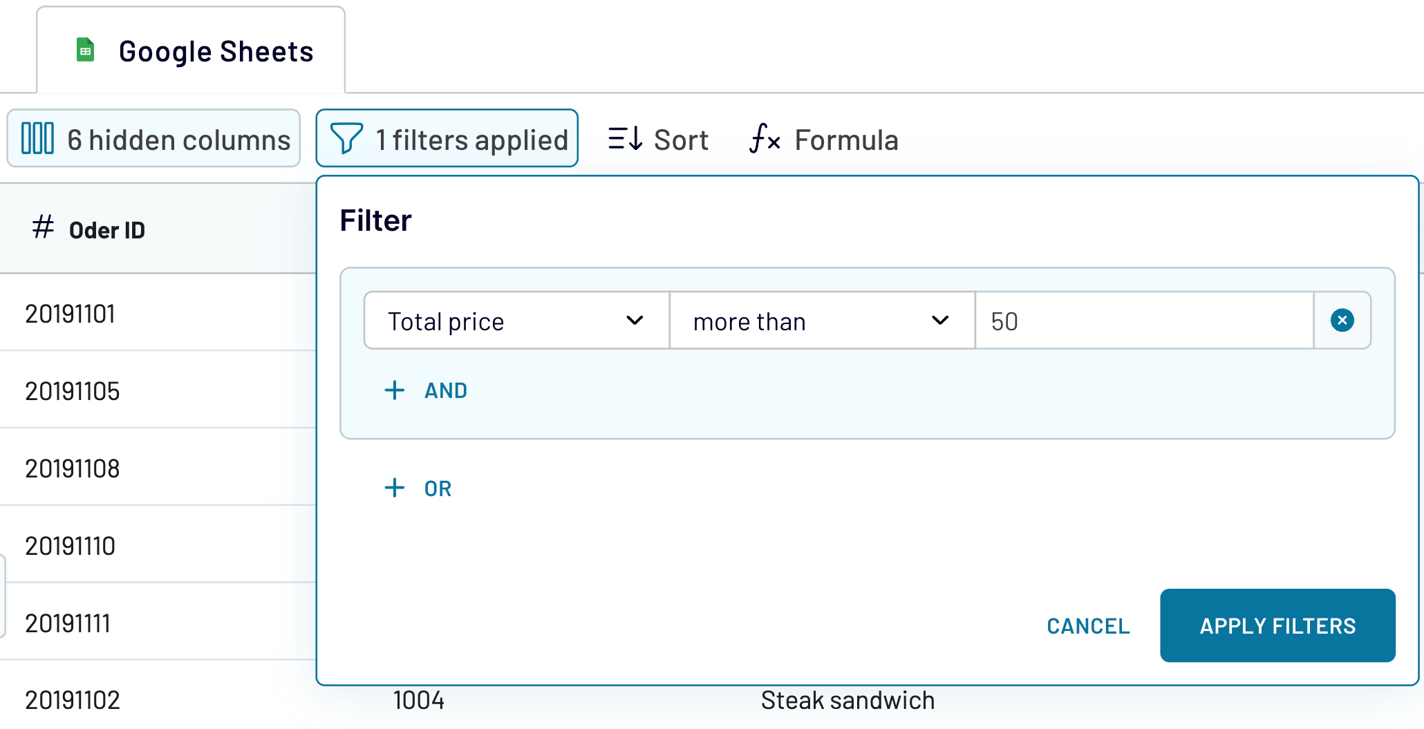
You can use filtering and other query options. Click Filter to filter out the products with a total price of more than $50. Select the column named Total price, specify the condition “more than”, and enter 50 in the value field.
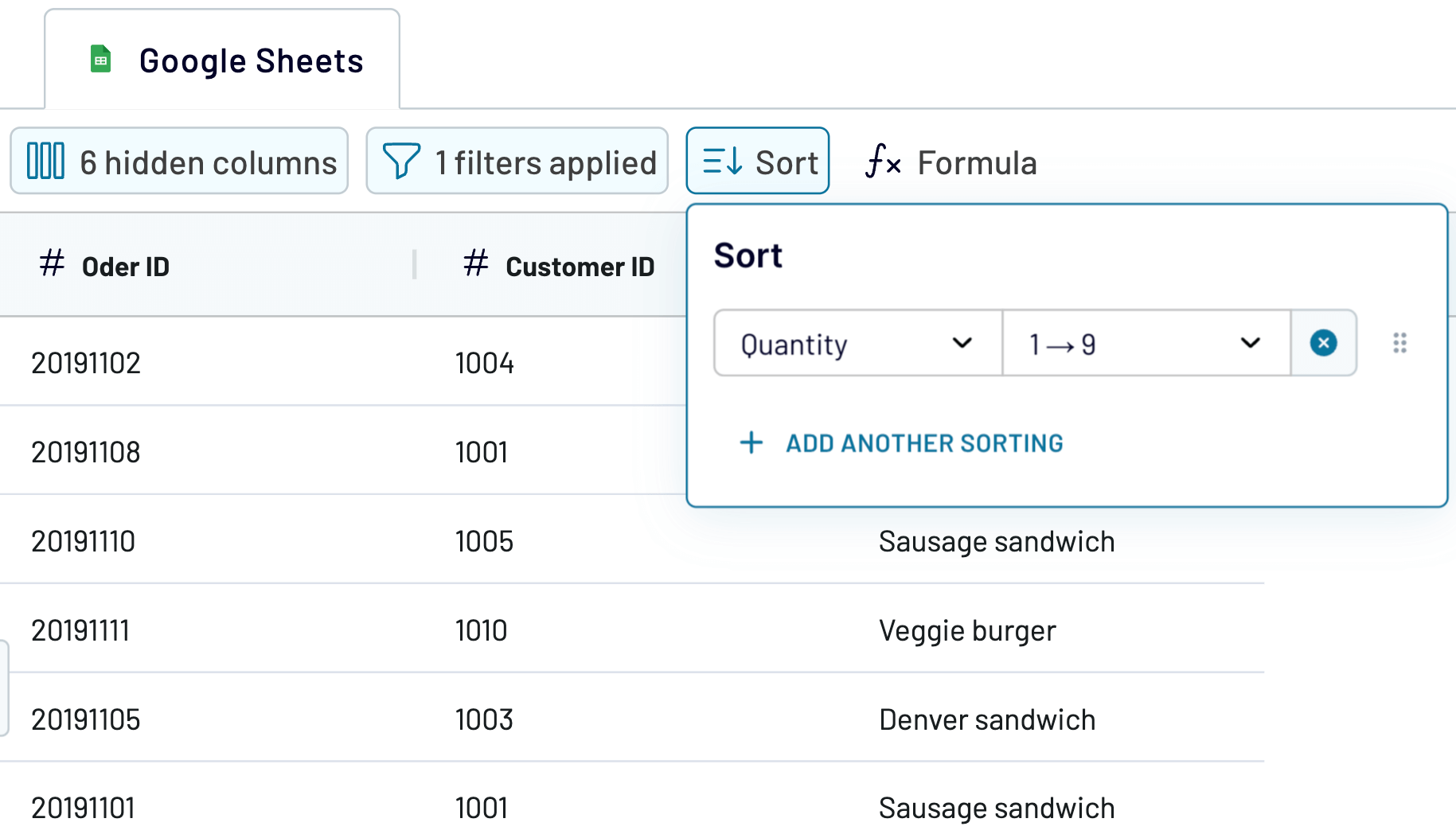
Click the Sort button, select the Quantity column, and choose ascending order.
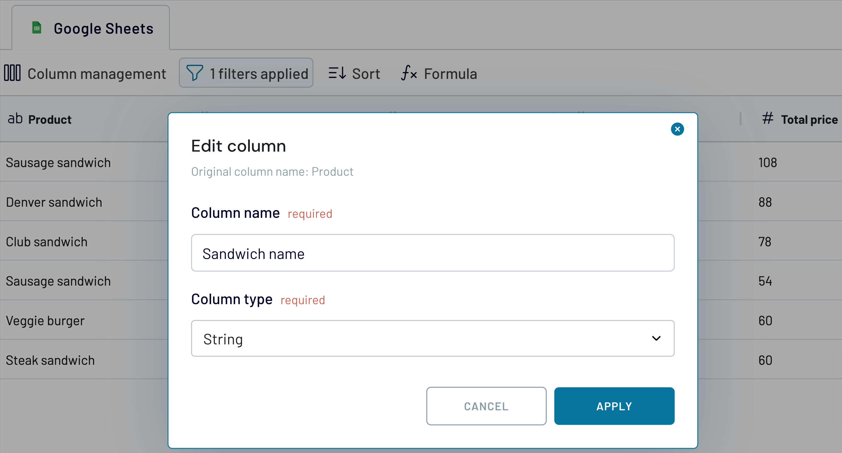
To change the header of the A column from “Product” to “Sandwich name”, click the three lines next to the column name and select Edit column.
Once your data is transformed, proceed to the destination settings for your data. You’ll need to choose the file and sheet where to import the queried data. Eventually, click Run importer.
Now you have your data available in the destination spreadsheet:
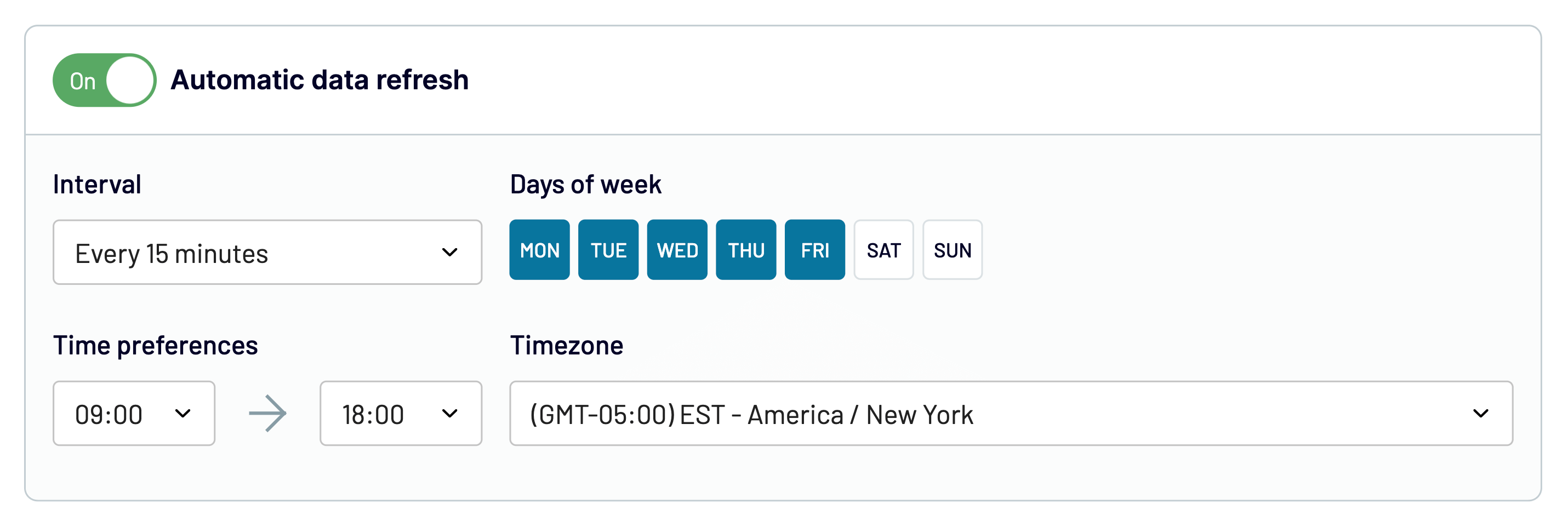
Optionally, turn on the Automatic data refresh and set your schedule for updates.

Automate data export with Coupler.io
Get started for freeWhat you can do with IMPORTRANGE+QUERY functions (real-life formula examples)
Now, let’s discover what a combination of IMPORTRANGE and QUERY can provide. Orders from Airtable will be our data source spreadsheet. All the rest is the magic of QUERY language clauses.
1. Import a specific range of data with the select QUERY clause
The select QUERY clause allows you to choose exactly which columns you want to pull. Check out more about Google Sheets Query: Select.
Task:
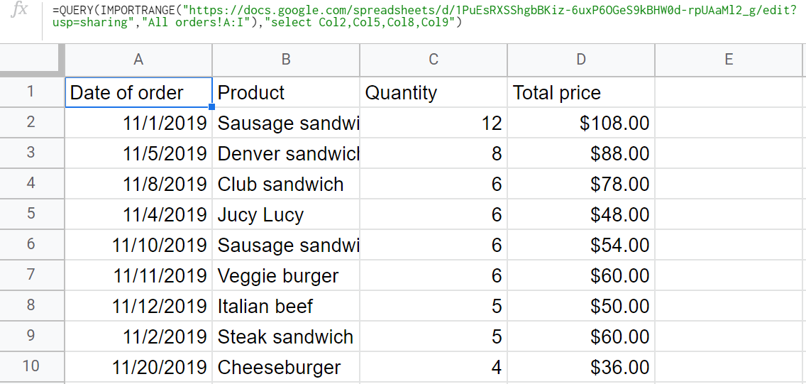
- Import columns B, E, H and I from the spreadsheet, Orders from Airtable.
QUERY+IMPORTRANGE formula example
=QUERY(IMPORTRANGE("https://docs.google.com/spreadsheets/d/1PuEsRXSShgbBKiz-6uxP6OGeS9kBHW0d-rpUAaMl2_g/edit?usp=sharing","All orders!A:I"),
  "select Col2,Col5,Col8,Col9")
You can check out the formula example in this tab.
2. Combine data from multiple sheets with QUERY and IMPORTRANGE
Now, chances are you may have data in several sheets and may want to merge certain information into a single sheet. No problem. You can also use QUERY and IMPORTRANGE with multiple sheets.
For this, use the same structure as we used before. However, you’ll need to wrap several IMPORTRANGE functions in curly braces {} and separate them by either commas (to merge data horizontally) or semicolons (to merge data vertically).
QUERY + IMPORTRANGE formula syntax to merge spreadsheets horizontally:
=QUERY({IMPORTRANGE("spreadsheet1_url", "data_range"),IMPORTRANGE("spreadsheet2_url", "data_range"),IMPORTRANGE("spreadsheet3_url", "data_range"),..}, "query_string")
QUERY + IMPORTRANGE formula syntax to merge spreadsheets vertically:
=QUERY({IMPORTRANGE("spreadsheet1_url"; "data_range"),IMPORTRANGE("spreadsheet2_url"; "data_range"),IMPORTRANGE("spreadsheet3_url"; "data_range");..}, "query_string")
data_range must contain the same column range for each spreadsheet_url, whereas the number of rows may differ.
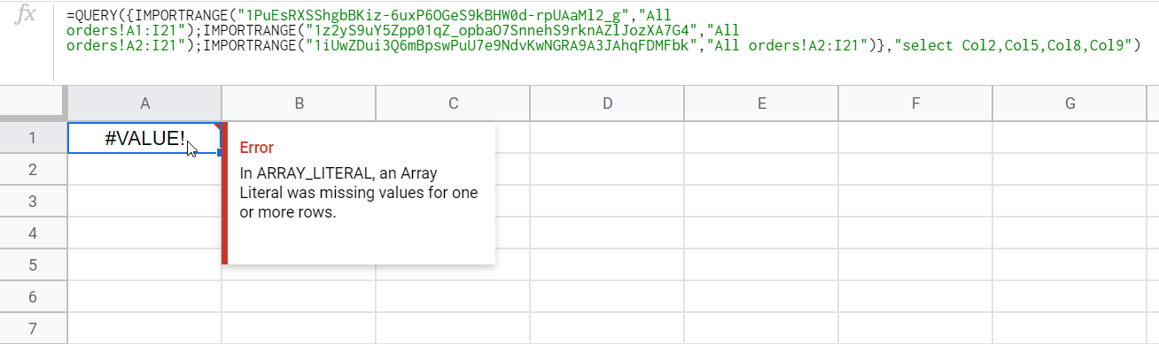
IMPORTANT: Before importing data from multiple sheets with QUERY and IMPORTRANGE, you’ll have to make data imports from each spreadsheet separately to allow access. Otherwise, you’ll get #VALUE! Error:in ARRAY_LITERAL, an Array Literal was missing values for one or more rows.
The reason is quite simple: when you IMPORTRANGE data from a particular spreadsheet for the first time, the formula requests to allow access: you need to click on a small button that pops up from the cell.
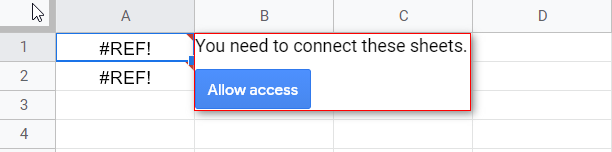
But there is no such button when you do it for several sources. Check out our blog post Why IMPORTRANGE Is Not Working to handle other errors.
Task:
- Import columns B, E, H and I from the spreadsheet#1, Orders from Airtable.
- Import columns B, E, H and I from the spreadsheet#2, Orders from Airtable#2.
- Import columns B, E, H and I from the spreadsheet#3, Orders from Airtable#3.
- Skip the first row when exporting data from spreadsheets #2 and #3.
QUERY+IMPORTRANGE formula example
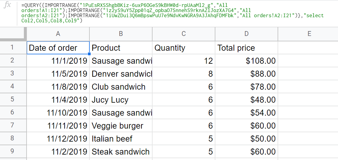
=QUERY({IMPORTRANGE("1PuEsRXSShgbBKiz-6uxP6OGeS9kBHW0d-rpUAaMl2_g","All orders!A1:I21"); IMPORTRANGE("1z2yS9uY5Zpp01qZ_opbaO7SnnehS9rknAZlJozXA7G4","All orders!A2:I21"); IMPORTRANGE("1iUwZDui3Q6mBpswPuU7e9NdvKwNGRA9A3JAhqFDMFbk","All orders!A2:I21")},
"select Col2,Col5,Col8,Col9")
Once we allowed access to the final spreadsheet, our formula for multiple sources immediately worked.
You can check out the formula example in this tab.
3. Cut off unnecessary rows of the imported data with the limit and offset QUERY clauses
The limit QUERY clause allows you to define the total number of rows (excluding the header) to be imported. The offset QUERY clause allows you to define how many rows to cut off from the top of the imported data range. Check out more about Google Sheets Query: Limit and Offset.
Task #1:
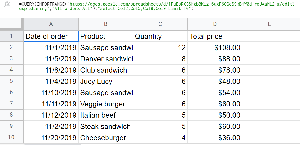
- Import columns B, E, H and I from the spreadsheet, Orders from Airtable.
- Reduce the number of imported rows to 10 (excluding the header).
QUERY+IMPORTRANGE formula example:
=QUERY(IMPORTRANGE("https://docs.google.com/spreadsheets/d/1PuEsRXSShgbBKiz-6uxP6OGeS9kBHW0d-rpUAaMl2_g/edit?usp=sharing","All orders!A:I"),
  "select Col2,Col5,Col8,Col9 Limit 10")
You can check out the formula example in this tab.
Task #2:
- Import columns B, E, H and I from the spreadsheet, Orders from Airtable.
- Reduce the number of imported rows to 10 (excluding the header).
- Skip five rows from the top of the spreadsheet we export data from (excluding the header).
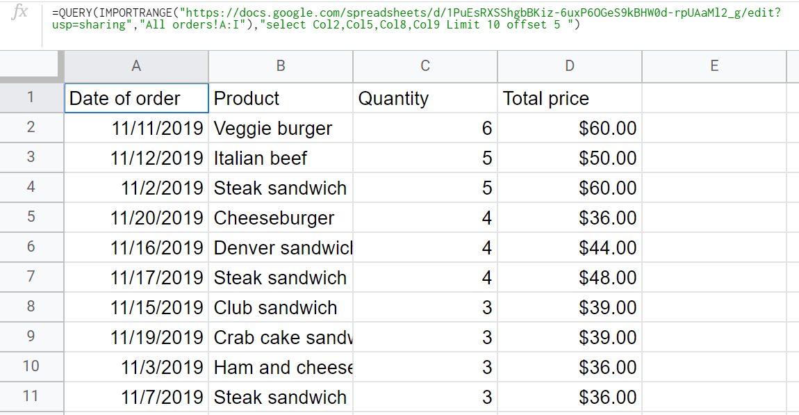
QUERY+IMPORTRANGE formula example:
=QUERY(IMPORTRANGE("https://docs.google.com/spreadsheets/d/1PuEsRXSShgbBKiz-6uxP6OGeS9kBHW0d-rpUAaMl2_g/edit?usp=sharing","All orders!A:I"),
  "select Col2,Col5,Col8,Col9 Limit 10 offset 5")
You can check out the formula example in this tab.
4. Change names of the imported columns with the label QUERY clause
The label QUERY clause allows you to change columns’ names (headers). Check out more about Google Sheets Query: Label.
Task:
- Import columns B, E, H and I from the spreadsheet, Orders from Airtable.
- Reduce the number of imported rows to 10 (excluding the header).
- Rename the headers of the imported columns:
- Date of order => Time
- Product => Sandwich
- Quantity => How many
- Total price => How much
QUERY+IMPORTRANGE formula example
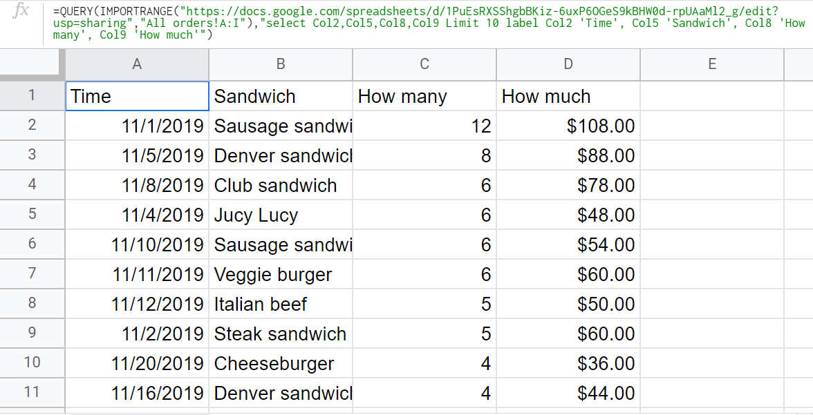
=QUERY(IMPORTRANGE("https://docs.google.com/spreadsheets/d/1PuEsRXSShgbBKiz-6uxP6OGeS9kBHW0d-rpUAaMl2_g/edit?usp=sharing","All orders!A:I"),
  "select Col2,Col5,Col8,Col9 Limit 10 label Col2 'Time', Col5 'Sandwich', Col8 'How many', Col9 'How much'")
You can check out the formula example in this tab.
5. Format values in the imported columns with the format QUERY clause
The format QUERY clause allows you to apply specific formats to imported columns. Check out more about Google Sheets Query: Format.
Task:
- Import columns B, E, H and I from the spreadsheet, Orders from Airtable.
- Reduce the number of imported rows to 10 (excluding the header).
- Format values in the B column to display month and year only.
QUERY+IMPORTRANGE formula example
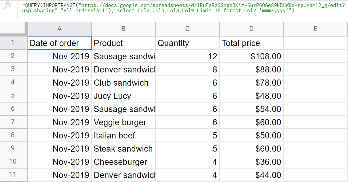
=QUERY(IMPORTRANGE("https://docs.google.com/spreadsheets/d/1PuEsRXSShgbBKiz-6uxP6OGeS9kBHW0d-rpUAaMl2_g/edit?usp=sharing","All orders!A:I"),
  "select Col2,Col5,Col8,Col9 Limit 10 format Col2 'mmm-yyyy'")
You can check out the formula example in this tab.
6. Import the filtered data with the where QUERY clause
The where QUERY clause allows you to filter rows in the imported columns based on set conditions. Check out more about Google Sheets Query: Where.
Task:
- Import columns B, E, H and I from the spreadsheet Orders from Airtable.
- Filter the imported data by the following conditions – the value in column I should be greater than or equal to 50.
QUERY+IMPORTRANGE formula example
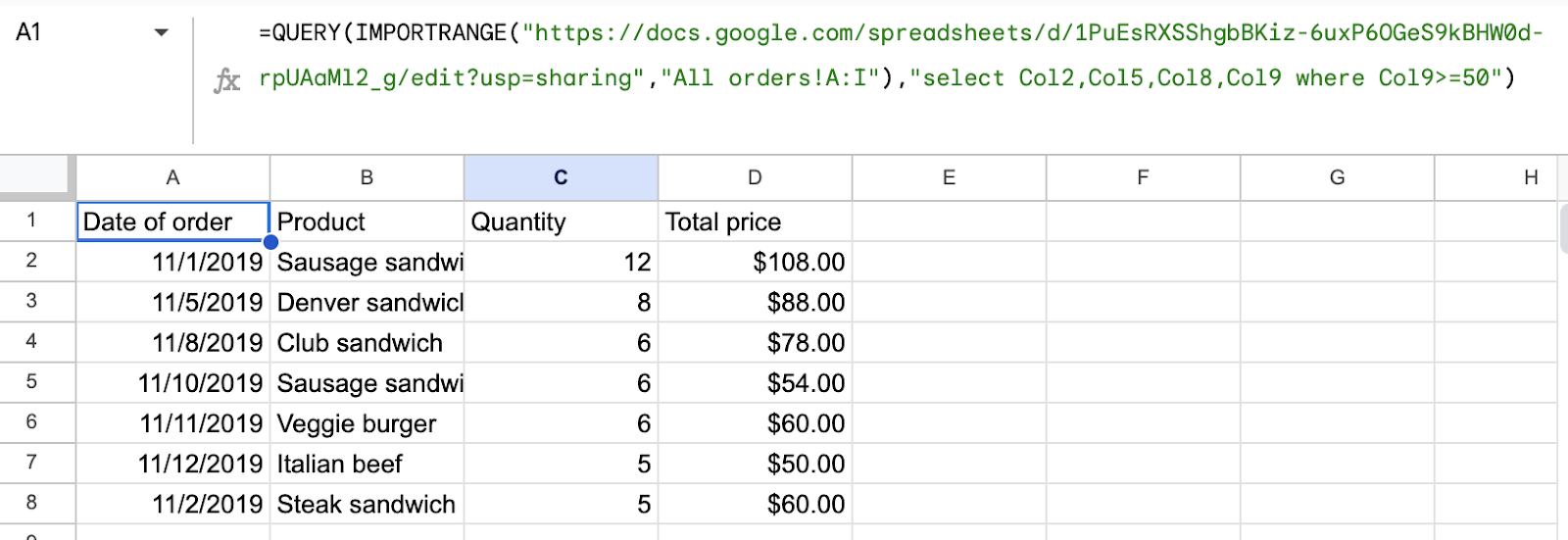
=QUERY(IMPORTRANGE("https://docs.google.com/spreadsheets/d/1PuEsRXSShgbBKiz-6uxP6OGeS9kBHW0d-rpUAaMl2_g/edit?usp=sharing","All orders!A:I"),
  "select Col2,Col5,Col8,Col9 where Col9>=50")
7. Apply multiple criteria for QUERY and IMPORTRANGE
Continuing with the previous example – when using the where statement you don’t need to limit yourself to a single criterion. Using operators like and or or you can filter for multiple criteria using QUERY and IMPORTRANGE.
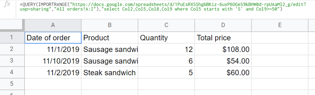
Task:
- Filter the earlier formula to also fetch orders where the value in column E starts with the letter “S”.
QUERY+IMPORTRANGE formula example
=QUERY(IMPORTRANGE("https://docs.google.com/spreadsheets/d/1PuEsRXSShgbBKiz-6uxP6OGeS9kBHW0d-rpUAaMl2_g/edit?usp=sharing","All orders!A:I"),"select Col2,Col5,Col8,Col9 where Col5 starts with 'S' and Col9>=50")
You can check out the formula example in this tab.
What’s more, you can also use QUERY and IMPORTRANGE with multiple criteria and an or operator to select results that meet either of the criteria. For example:
=QUERY(IMPORTRANGE("https://docs.google.com/spreadsheets/d/1PuEsRXSShgbBKiz-6uxP6OGeS9kBHW0d-rpUAaMl2_g/edit?usp=sharing","All orders!A:I"),"select Col2,Col5,Col8,Col9 where Col5 starts with 'S' or Col9<30")
8. Find data that contains a certain phrase using QUERY and IMPORTRANGE
You can also use the where clause to specify what a certain column should contain to meet your criteria or what phrase to avoid when returning results. For that, you use a contains operator.
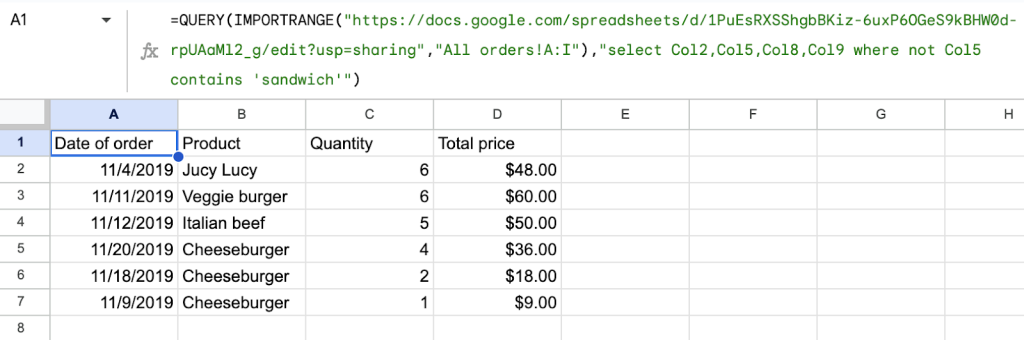
Task:
- Filter the order data to fetch only the orders with products that don’t contain the word “sandwich”
QUERY+IMPORTRANGE formula example:
=QUERY(IMPORTRANGE("https://docs.google.com/spreadsheets/d/1PuEsRXSShgbBKiz-6uxP6OGeS9kBHW0d-rpUAaMl2_g/edit?usp=sharing","All orders!A:I"),"select Col2,Col5,Col8,Col9 where not Col5 contains 'sandwich'")
To find data that contains a certain phrase in QUERY + IMPORTRANGE, skip the not keyword.
Note that the string you use with contains is case-sensitive. If you, for example, have both ‘Sandwich’ and ‘sandwich’ in the table, you’ll want to use or or and operators to pick either of these versions, repeating the whole ‘contains’ statement. For example:
where not Col5 contains 'sandwich' and not Col5 contains 'Sandwich'
where Col5 contains 'sandwich' or Col5 contains 'Sandwich'
9. Sort the imported data with the order by QUERY clause
The order by QUERY clause allows you to sort data based on the chosen column in ascending/descending order. Check out more about Google Sheets Query: Order By.
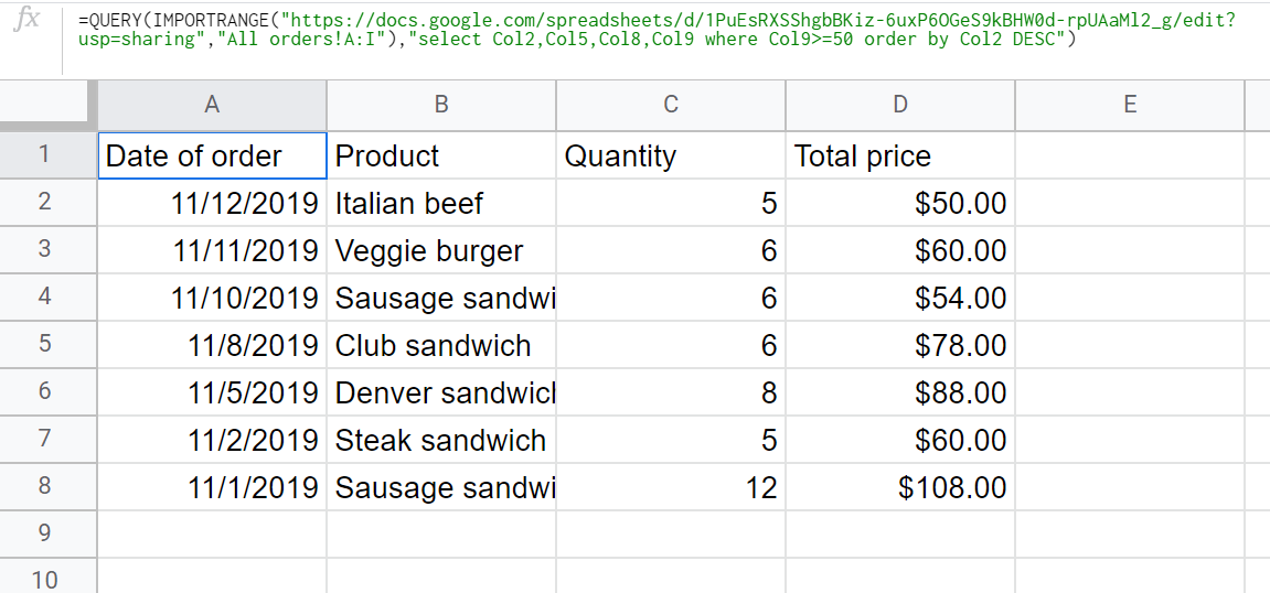
Task:
- Import columns B, E, H and I from the spreadsheet, Orders from Airtable.
- Filter the imported data by the column I where the values should be greater than or equal to 50.
- Sort the imported data by the date of order (column B) in descending order
QUERY+IMPORTRANGE formula example
=QUERY(IMPORTRANGE("https://docs.google.com/spreadsheets/d/1PuEsRXSShgbBKiz-6uxP6OGeS9kBHW0d-rpUAaMl2_g/edit?usp=sharing","All orders!A:I"),
  "select Col2,Col5,Col8,Col9 where Col9>=50 order by Col2 DESC")
You can check out the formula example in this tab.
10. Arithmetic operations with the imported data
You can add (+), subtract (-), multiply (*), and divide (/) columns from a spreadsheet and import the outcome as a separate column. Check out more about Google Sheets Query: Arithmetic Operators.
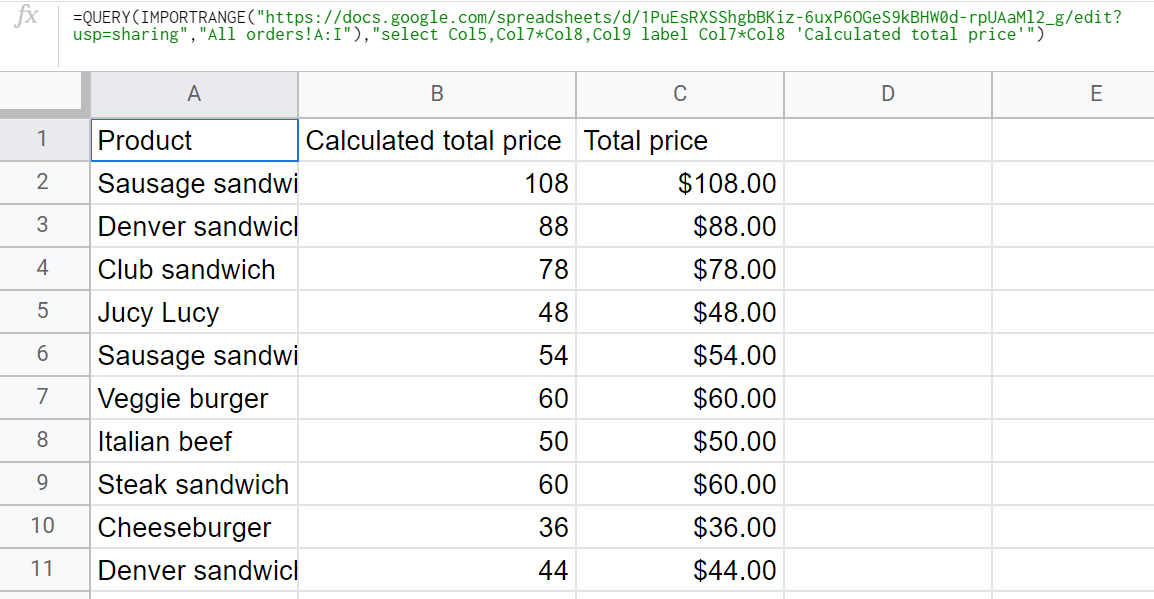
Task:
- Import columns E and I from the spreadsheet Orders from Airtable.
- Multiply the Price (column G) by the Quantity (column H) and import the outcome as a separate column named “Calculated total price”.
QUERY+IMPORTRANGE formula example
=QUERY(IMPORTRANGE("https://docs.google.com/spreadsheets/d/1PuEsRXSShgbBKiz-6uxP6OGeS9kBHW0d-rpUAaMl2_g/edit?usp=sharing","All orders!A:I"),
  "select Col5,Col7*Col8,Col9 label Col7*Col8 'Calculated total price'")
You can check out the formula example in this tab.
11. Aggregation operations with the imported data
Within the select, order by, label, and format QUERY clauses, you can apply the following aggregation functions to the imported columns:
avg()– provides the average of all numbers in a column.sum()– provides the sum of all numbers in a column.count()– provides the quantity of items in a column (rows with empty cells are not calculated).max()– provides the maximum value in a column.min()– provides the minimum value in a column.
Aggregation functions are not applicable to where, group by, pivot, limit and offset QUERY clauses.
Check out more about Google Sheets Query: Aggregation Functions.
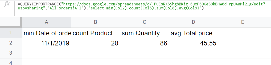
Task:
- Import columns B, E, H and I from the spreadsheet, Orders from Airtable.
- Provide the minimum value in column B.
- Count the items in column E.
- Provide the sum of all numbers in column H.
- Provide the average of all values in column I.
QUERY+IMPORTRANGE formula example
=QUERY(IMPORTRANGE("https://docs.google.com/spreadsheets/d/1PuEsRXSShgbBKiz-6uxP6OGeS9kBHW0d-rpUAaMl2_g/edit?usp=sharing","All orders!A:I"),
  "select min(Col2),count(Col5),sum(Col8),avg(Col9)")
You can check out the formula example in this tab.
12. Scalar operations with the imported data
You can use scalar functions to convert imported parameters into a single value. For example, if you apply the year() scalar function, it will fetch the year value out of the YYYY-MM-DD format. Check out more about Google Sheets Query: Scalar Functions.
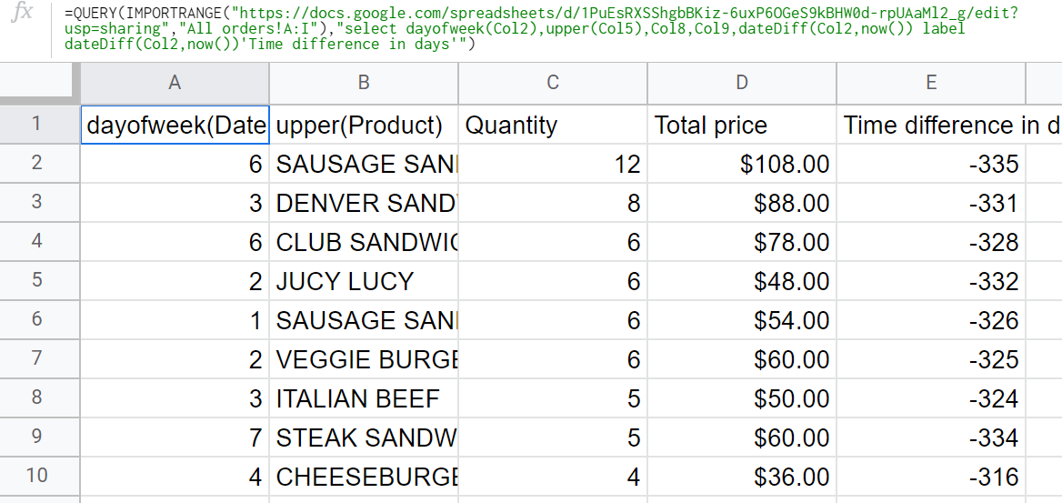
Task:
- Import columns B, E, H and I from the spreadsheet, Orders from Airtable.
- Fetch the day of the week from date values in column B.
- Replace all the letters with uppercase ones in column E.
- Calculate the difference between the date of order and current time, and import the values in a separate column named “Time difference in days”.
QUERY+IMPORTRANGE formula example
=QUERY(IMPORTRANGE("https://docs.google.com/spreadsheets/d/1PuEsRXSShgbBKiz-6uxP6OGeS9kBHW0d-rpUAaMl2_g/edit?usp=sharing","All orders!A:I"),
  "select dayofweek(Col2),upper(Col5),Col8,Col9,dateDiff(Col2,now()) label dateDiff(Col2,now())'Time difference in days'")
You can check out the formula example in this tab.
13. Aggregate the imported data across rows with the group by QUERY clause
The group by QUERY clause allows you to group values across the selected data range based on a specific condition. The clause can be applied if an aggregation function has been used within the select clause. Check out more about Google Sheets Query: Group By.
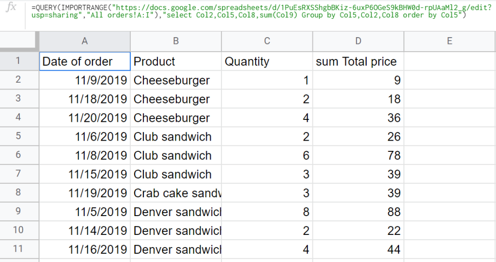
Task:
- Import columns B, E, H and I from the spreadsheet, Orders from Airtable.
- Summarize the Total price data (column I).
- Group the aggregated values by the Product name (column E).
- Sort the imported data by the grouped values (column E) in ascending order.
QUERY+IMPORTRANGE formula example
=QUERY(IMPORTRANGE("https://docs.google.com/spreadsheets/d/1PuEsRXSShgbBKiz-6uxP6OGeS9kBHW0d-rpUAaMl2_g/edit?usp=sharing","All orders!A:I"),
  "select Col2,Col5,Col8,sum(Col9) Group by Col5,Col2,Col8 order by Col5")
You can check out the formula example in this tab.
14. Aggregate the imported data and rotate rows into columns with the pivot QUERY clause
The pivot QUERY clause allows you to convert rows into columns, and vice versa, as well as aggregate, transform and group data by any field. The clause can be applied if an aggregation function has been used within the select QUERY clause. Check out more about Google Sheets Query: Pivot.
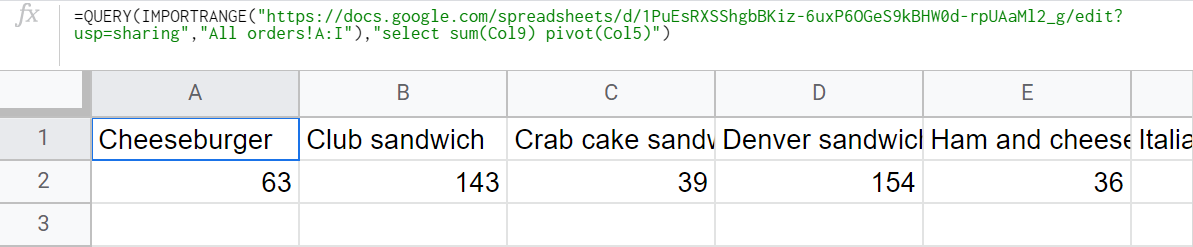
Task:
- Import columns E and I from the spreadsheet Orders from Airtable.
- Summarize the Total price data (column I).
- Pivot the aggregated values by the Product name (column E).
QUERY+IMPORTRANGE formula example
=QUERY(IMPORTRANGE("https://docs.google.com/spreadsheets/d/1PuEsRXSShgbBKiz-6uxP6OGeS9kBHW0d-rpUAaMl2_g/edit?usp=sharing","All orders!A:I"),
  "select sum(Col9) pivot(Col5)")
You can check out the formula example in this tab.
Try the QUERY and IMPORTRANGE alternative to query your data without formulas
Well, this was a pretty long journey, but you handled it! Now you know everything you can do with QUERY and IMPORTRANGE in Google Sheets. Still, these formulas might not be easy to use, taking much time and putting you at risk of syntax errors.
That’s why, for more advanced cases, you’d better take a no-formula approach by using Coupler.io. It can help you query your data range from other spreadsheets or external sources and load it to the needed spreadsheet. So, give it a try, and you won’t have to spend time on formulas or ever get #ERROR anymore 🙂
Automate data export with Coupler.io
Get started for free