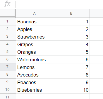
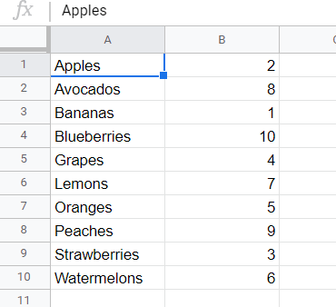
Here is a spreadsheet with the most popular fruits in the U.S. listed by popularity:
What we want to do is sort this data in alphabetical order. Since it’s a simple use case, a couple of mouse clicks will do the job. However, what if you have a larger data set and more advanced sorting needs? Read this blog post to learn everything about sorting data in Google Sheets.
Import and sort data in Google Sheets without formulas
If you’re loading your data from external sources into Google Sheets, you can automate this process and sort data on the go with the help of Coupler.io.
Coupler.io is a data automation and analytics platform that allows you to automate data import into Google Sheets (and other destinations) from multiple apps (Shopify, Airtable, Xero, etc.) and databases. Before loading your source data to the target spreadsheet, you can perform versatile transformations including sorting by one or multiple columns. This can be done easily in any of Coupler.io’s Google Sheets integrations without any formulas. Here is what it may look like in the example of Shopify to Google Sheets integration:
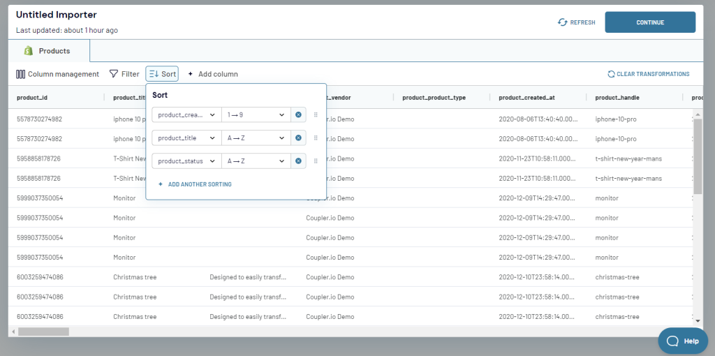
To start using the tool, sign up to Coupler.io or install Coupler.io Google Sheets add-on from the Google Workspace Marketplace.
Now let’s see the native options you can consider to sort data in Google Sheets.
How to sort all data in Google Sheets by alphabet
Google Sheets provides two built-in options to sort data alphabetically:
- Sort sheet – sorts all data on the sheet by a specific column.
- Sort range – sorts the data in a selected range by a specific column.
You can find both options in the Data menu.
Let’s use them to handle our task – sorting the list of fruits from A to Z.
Sort sheet by a column in Google Sheets
To sort the entire sheet, take the following steps:
- Select the column to sort by. To do this, select any cell of the required column.
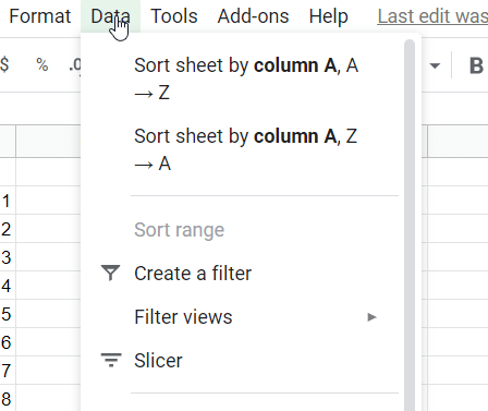
- Go to the Data menu and select the alphabetical order for sorting:
- Sort sheet by
{selected-column}, A to Z - Sort sheet by
{selected-column}, Z to A
- Sort sheet by
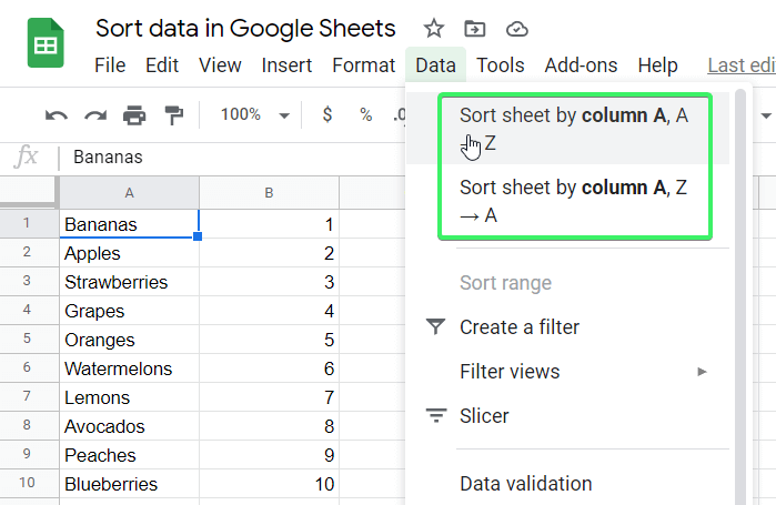
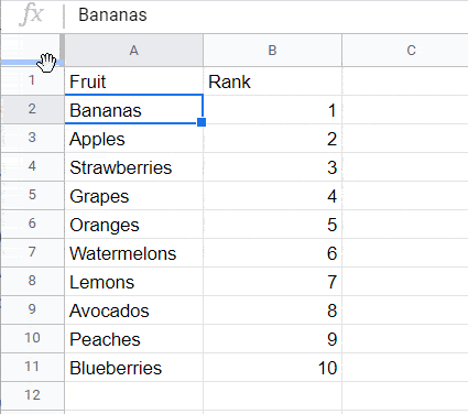
Let’s sort our list of fruits from A to Z – here is what it looks like:
How to sort data in Google Sheets with a header row
If your data set has a header row, freeze it before sorting. To do this, click and drag the grey horizontal line that you can find in the top-left corner of the spreadsheet.
Note: If you skip this, the Sort sheet function will include the header row in the sorting.
Now you can apply the Sort sheet option as it was described above.
How to sort data in Google Sheets by range
The second built-in option, Sort range, also lets you sort data alphabetically. However, it sorts the data range you select rather than the entire sheet:
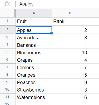
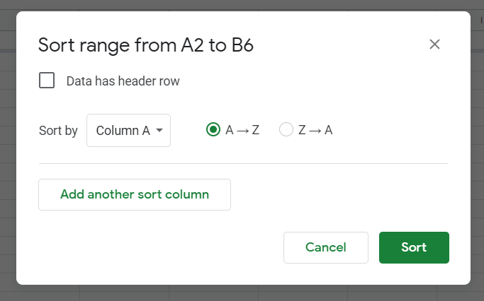
- Select the range you want to sort. For example, let’s sort the range
A2:B6.
- Go to the Data menu and select the alphabetical order for sorting the selected range:
- Sort range by
{selected-column}, A to Z - Sort range by
{selected-column}, Z to A
- Sort range by
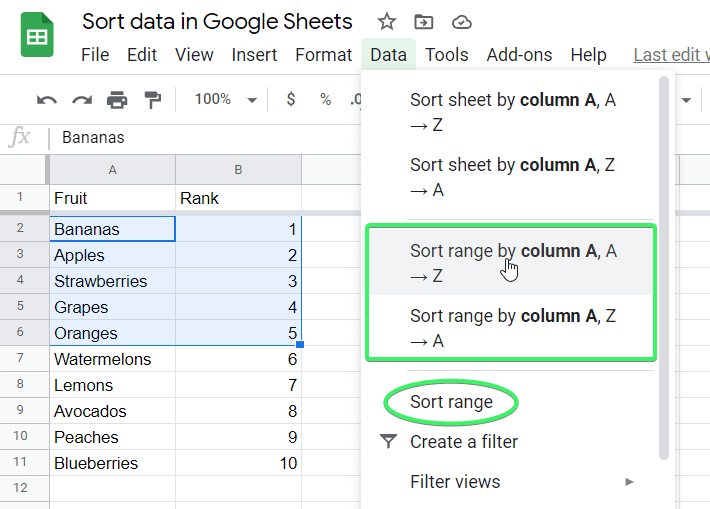
Alternatively, you can click Sort range and configure the sorting there:
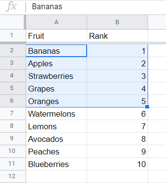
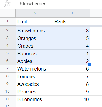
Take a look at what the data range looks like if sorted in reverse alphabetical order, Z to A:
How to sort by value in Google Sheets
Sorting means to order data in an increasing or decreasing manner. So, technically, you can’t sort by value. Instead, you can filter data by value. This is where the confusion between sorting and filtering by comes from.
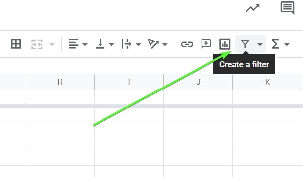
If you need to filter data by value, click the Create a filter button.
Then click the hamburger menu on the column you want to filter values by and select Filter by values.
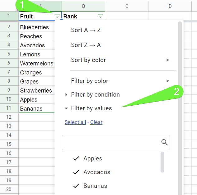
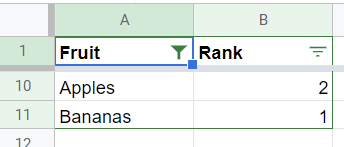
Specify one or several values to filter by and click Ok. The data set will be filtered accordingly.
Read our blog post to learn more about filtering in Google Sheets.
How to sort data by numerical value in Google Sheets
You can apply the mentioned sorting options to easily sort numerical values as well. Here is how it works.
How to sort data from lowest to highest in Google Sheets
- Select the column that contains numerical values to sort by. In our case, this is column B.
- Go to the Data menu and select the alphabetical order for sorting:
- Sort sheet by
{selected-column}, A to Z
- Sort sheet by
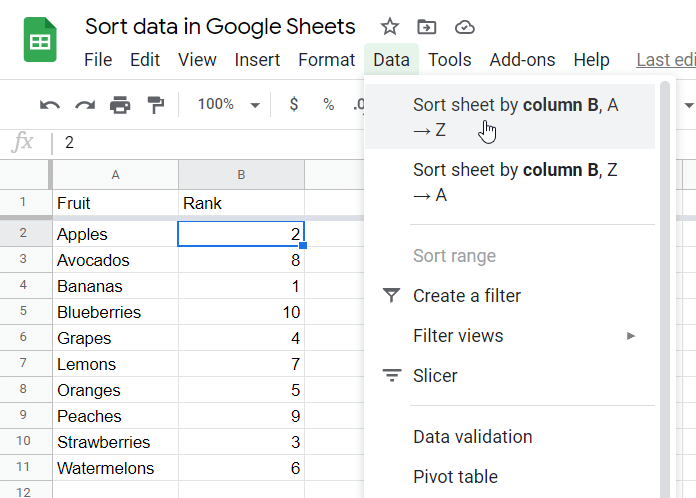
The data will be sorted by column B in ascending numeric order.
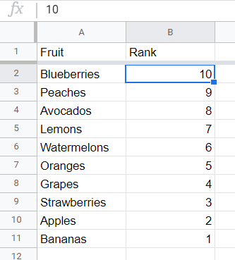
How to sort data from highest to lowest in Google Sheets
To change the sorting order to descending, use
- Sort sheet by
{selected-column}, Z to A.
There you go:
How to sort data in Google Sheets by two different columns
Now, our data set allows us to show you how you can sort data by multiple columns.
- Select the range and go to Data => Sort range
- Select the primary column to sort by, then click the button to Add another sort column
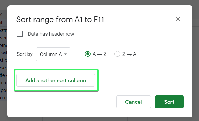
Click Sort once you’re ready to sort the data.
Note: You can sort data by multiple columns using the SORT function as well. We’ll talk about that a bit later.
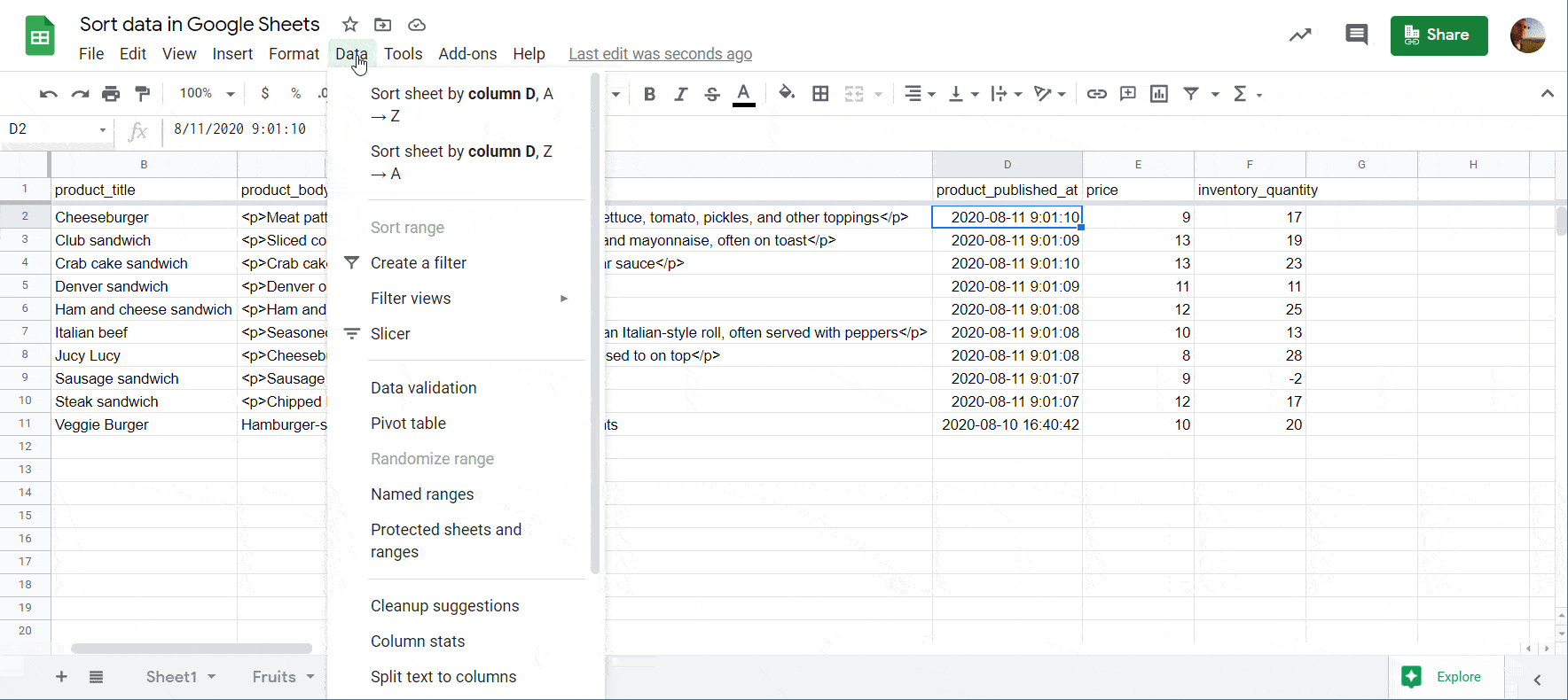
How to sort data by date in Google Sheets
In a similar way to using either Sort sheet or Sort range features, you can sort your data by date. In our example, we need to:
- Freeze the header row
- Select any cell in the D column (the column with date values)
- Go to Data => Sort sheet by column D, A – Z (for ascending order) or Sort sheet by column D, Z – A (for descending order)
How to sort data in Google Sheets without messing up formulas
We don’t know which formulas you have for the data set to sort, but here are the most common use cases of calculation errors when sorting.
ARRAYFORMULA calculations messed up after sorting
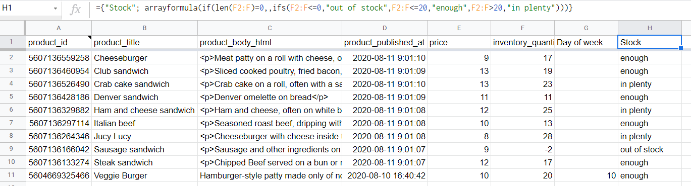
Quite often we apply array formulas not in the heading section. For example, here is the array formula in the H2 cell that shows the stock status:
=arrayformula(if(len(F2:F)=0,,
     ifs(
         F2:F<=0,"out of stock",
         F2:F<=20,"enough",
         F2:F>20,"in plenty"
     )
))
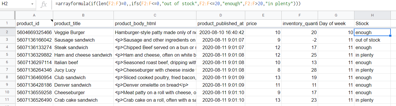
If we sort the data set, let’s say alphabetically by column B, the array formula will change its location and mess up.
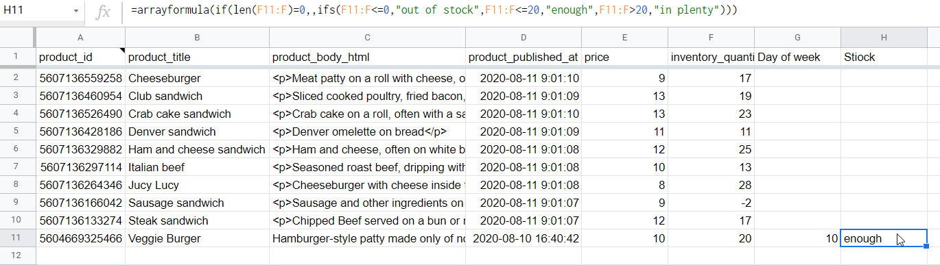
To avoid this, make sure to locate your array formulas in the header section, so that they won’t be ruined after sorting. Here is what it may look like in H1 cell:
={
   "Stock";
   arrayformula(if(len(F2:F)=0,,
      ifs(
         F2:F<=0,"out of stock",
         F2:F<=20,"enough",F2:F>20,
         "in plenty"
      )
   ))
}
Cell reference broken after sorting and messed up calculations
Let’s say on another sheet, you have a formula with the reference to your data set. In our example, we have a simple SUM formula that totals the number of sandwiches (products which names contain “sandwich“) in stock.
=SUM(
      'Shopify Importer'!F3,
      'Shopify Importer'!F5,
      'Shopify Importer'!F7,
      'Shopify Importer'!F8,
      'Shopify Importer'!F9,
      'Shopify Importer'!F10
)
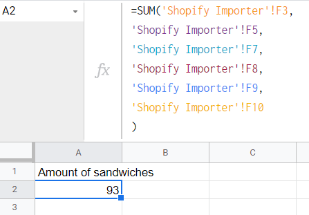
After sorting, as you understand, the calculation will mess up since the reference values will change. To avoid this, make sure to use certain criteria to reference the cells in the data set to be sorted. For this, you may benefit from such Google Sheets functions as QUERY, VLOOKUP, FILTER, and so on.
In our case, we can go with SUMIF. Here is the formula that filters values whose names contain “sandwich” and totals their amounts.
=sumif('Shopify Importer'!B2:B, "*sandwich*", 'Shopify Importer'!F2:F)
Regardless of how the data set is sorted, the sum remains stable compared to the use of the regular SUM formula.
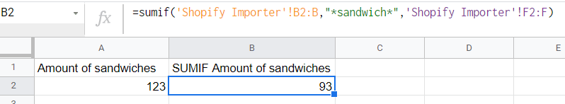
The idea here is to use more advanced formulas that will be independent of sorting.
How to sort data but keep blank rows in Google Sheets
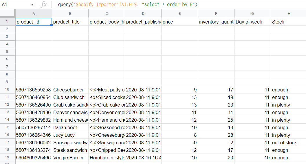
Another interesting case is with blank rows in a data set like this:
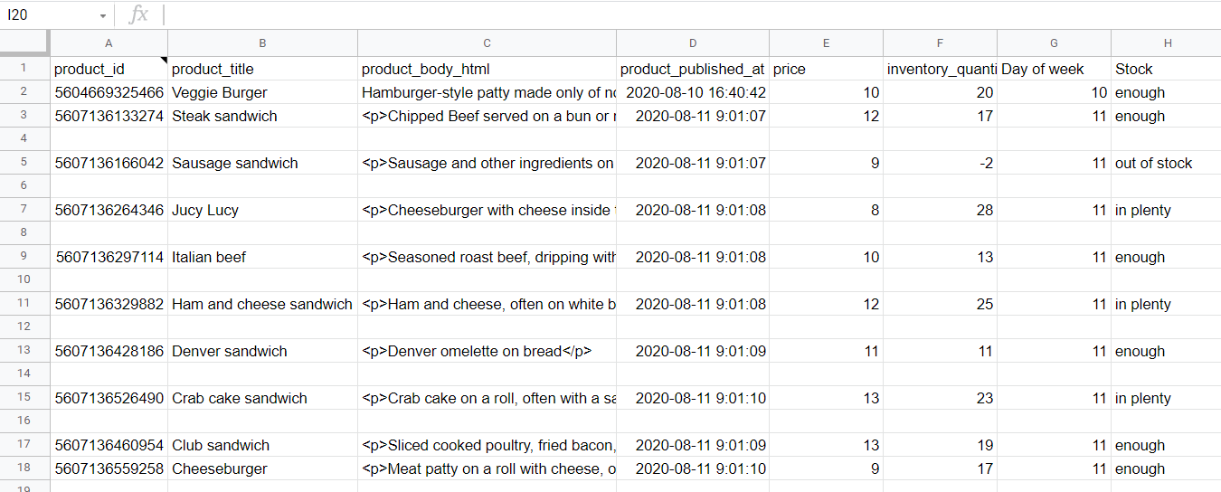
When you sort this data in Google Sheets, either in ascending or descending order, the blank rows always sink to the bottom. However, there is a way to make the blanks appear at the top of the data set when it is sorted. The QUERY Google Sheets function can do this. Here is what the formula should look like:
=query('Shopify Importer'!A1:H19, "select * order by B")
Shopify Importer'!A1:H19– the data range to sortorder by B– the column to sort the data by (you can choose any column)
There you go!
Since we touched upon using Google Sheets functions for sorting, let’s delve deeper into this.
Automatically sort data in Google Sheets using the SORT function
What does it mean to auto sort in Google Sheets?
The options described above are good for sorting static data – that is, every time you add new entries to your data set, you need to get it sorted manually. If you want to auto sort in Google Sheets, i.e. sort data dynamically, you should go with the SORT function. It is the Google Sheets function to sort data by the values in one or multiple columns. SORT doesn’t affect your current data set, but instead creates a newly sorted data set. Here is what the SORT syntax looks like:
=SORT(data-range, sort-column, ascending, sort-column2, ascending2, ...)data-range– the data range to sort.sort-column– the column to sort by (column index or a column range).sort-columncan be either within or outside thedata-range, but it must have the same number of rows as thedata-range.ascending– applyTRUEto sort in ascending order, orFALSEto sort in descending order.
Example of how to sort data dynamically in Google Sheets
Let’s auto sort our Shopify products in Google Sheets by price in descending order. To do this, we created a separate sheet and applied the following formula:
={
"id", "title", "description", "date", "price", "amount";
  	sort('Shopify Importer'!A2:F, 'Shopify Importer'!E2:E, false)
 }
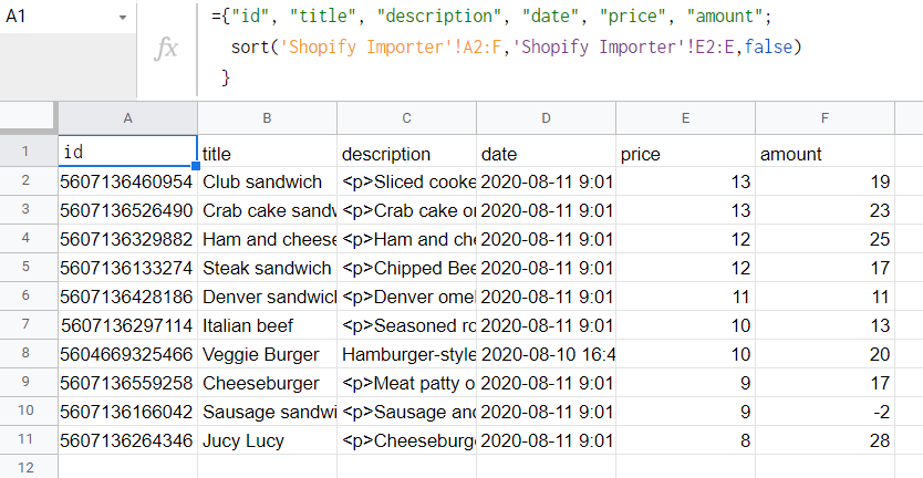
Now, every new row added to your data set will be automatically sorted.
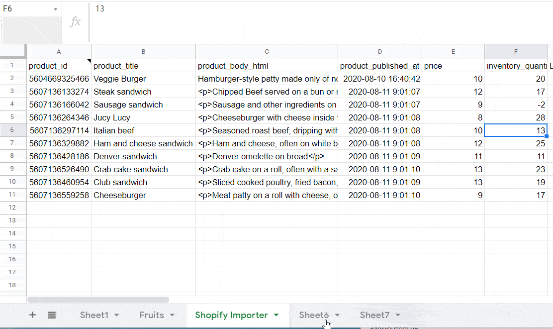
How to sort data in Google Sheets into different sheets
Using the SORT function, you can auto sort data into different Google sheets. To do this, you only need to specify the data range you want to place and sort to a specific sheet, and repeat this for other sheets. In our example, we may want to split the data set into two chunks and place them into two different sheets. So, we’ll need two SORT formulas for each sheet:
Sheet No. 1:
={
   "id", "title", "description", "date", "price", "amount";
   sort('Shopify Importer'!A2:F6, 5, false)
 }
'Shopify Importer'!A2:F6– first chunk of the data set5– the column index to sort by
Sheet No. 2:
={
   "id", "title", "description", "date", "price", "amount";
   sort('Shopify Importer'!A7:F11, 2, true)
 }
'Shopify Importer'!A7:F11– second chunk of the data set2– the column index to sort by
In this example, we split the data set into two chunks and sorted them differently in each sheet.

Reverse sort data in Google Sheets
It’s not a big deal to reverse the rows of your sorted data set. All you need to do is to change the sorting order from ascending to descending, or vice-versa. However, what if your data set is not sorted, and you do not want it sorted, just reversed?
In this case, you can reverse it using SORT quite easily. Here is the formula syntax to use:
=SORT(data-range,ROW(data-range),FALSE)In our example, the formula will look like this:
=SORT(A2:F11, ROW(A2:F11), FALSE)
or like this if you want to attach headers:
={
   "id", "title", "description", "date", "price", "amount";
   SORT(A2:F11, ROW(A2:F11), FALSE)
}
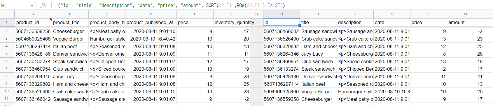
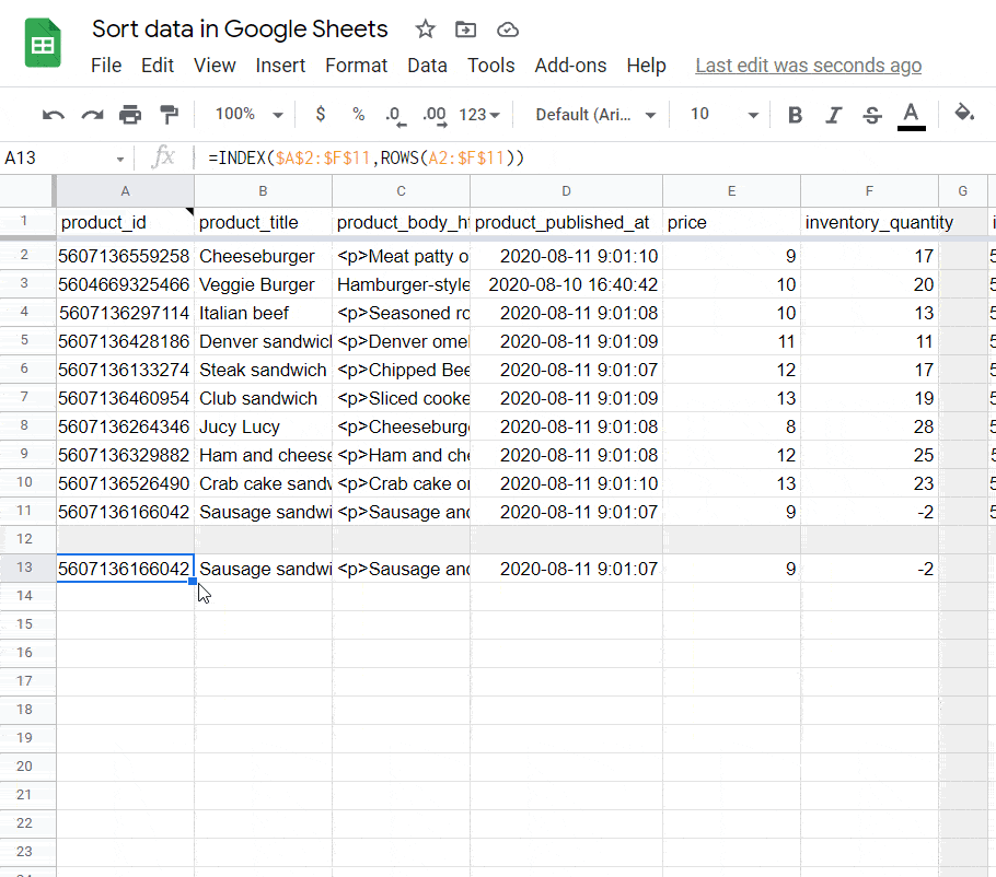
As an alternative, you may consider the use of the INDEX function nested with ROWS. The formula for our example will look as follows:
=INDEX($A$2:$F$11, ROWS(A2:$F$11))
This formula will return the last row of the data range. To get the rest ones, you’ll have to drag the formula down manually.
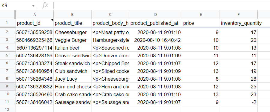
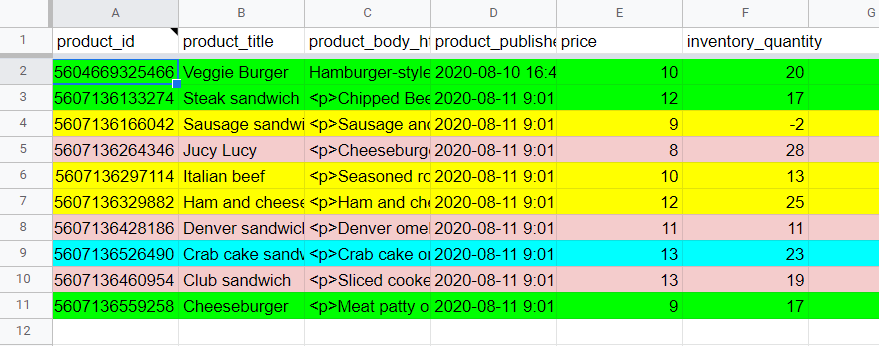
How to sort a data set by color in Google Sheets
Since 2020, Google Sheets users have a built-in functionality to sort data by color – both fill and text color. Let’s check out how it works in the example of the following data set.
To enable sorting by color, select any cell within the data range and click the filter button.
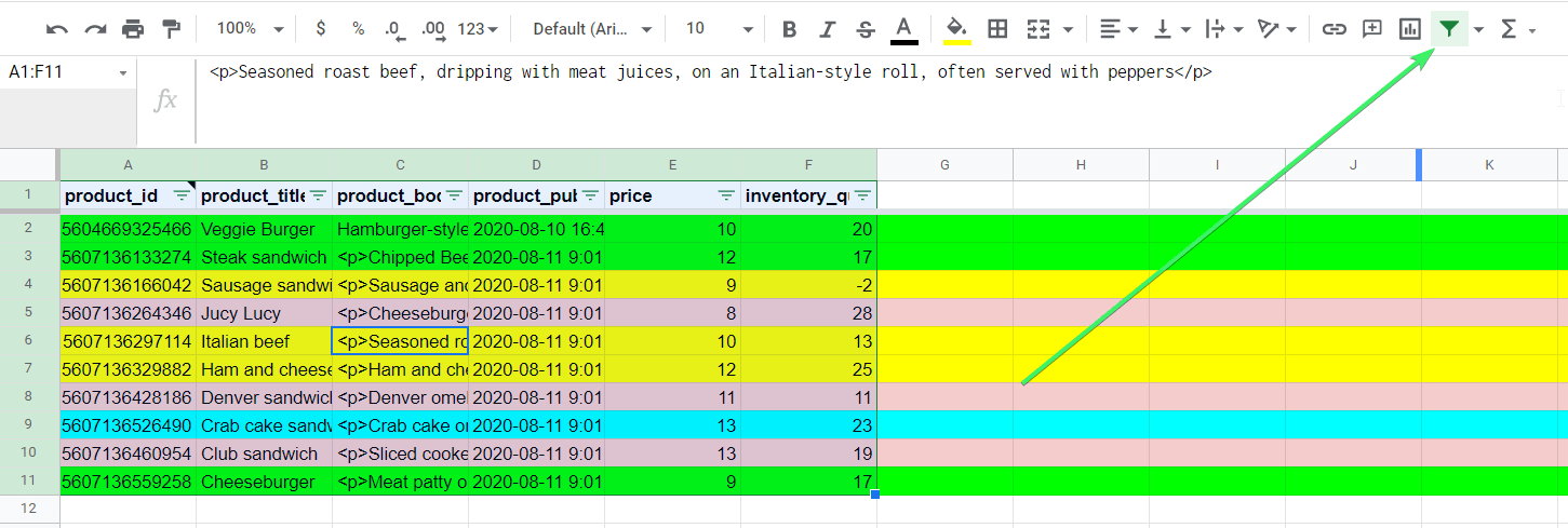
Now, click the filter icon next to the header for the column to sort by => Sort by color => Fill color => and select the color.
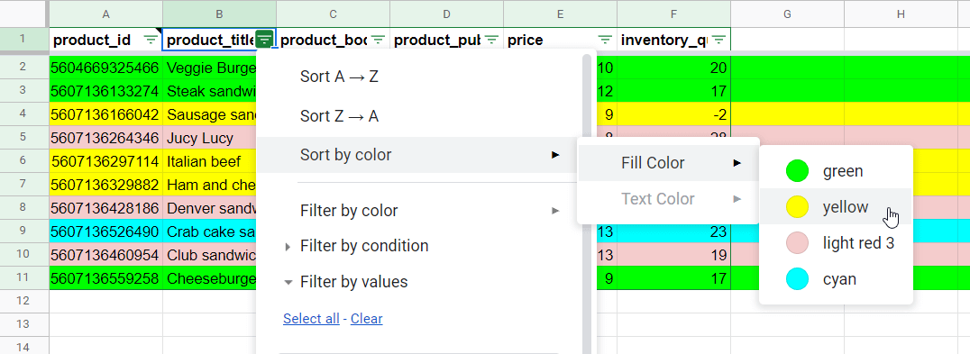
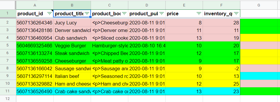
We selected yellow for our data range, and the sorting functionality now shows yellow colored rows first:
To group rows by color, you’ll need to repeat sorting for the rest of colors.
The same algorithm works when you need to sort data by text color.
To wrap up: How to sort rows in Google Sheets without mixing data
Previously, we introduced multiple options for you to sort your data without any mistakes. We do recommend that you use the SORT function in most cases, since it does not affect your existing data set when sorting. This will let you keep the raw data and the sorted data in separate sheets.
At the same time, the built-in sorting functionality in Google Sheets will do the job easier when you need to sort data right away. You probably know other ways to sort data without messing it up. Share your use cases with us and we’ll be happy to add them to this tutorial. Good luck with your data!