All or most of you know that you can filter data in Google Sheets using the filter button on the toolbar. It’s quite an actionable method, but it’s a manual one. So, you have to make a few clicks to make it work. If you want to automate filtering in Google Sheets, you’d better use the FILTER function. In this tutorial, we’ll explain how you can do this.
FILTER function Google Sheets explained
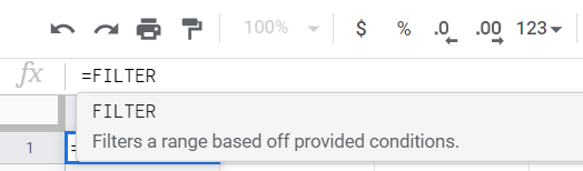
Google Sheets FILTER function filters out subsets of data from a specified data range by a provided condition.
The FILTER function and the filter functionality are different things. The function is used within formulas to filter subsets of data.
The functionality is a button on the toolbar of a spreadsheet. It filters the entire data set.
Google Sheets FILTER function syntax
=FILTER(data_range,condition_1, condition_2,...)
data_range– a range of cells to filter. Example:A2:A
condition– a cell range that contains TRUE or FALSE values of the filter criteria. The filter criteria mostly contains the comparison operators (“=“, “<“, and “>“), for example,A2:A>20. However, you can also use the REGEXMATCH function in the FILTER condition.
If a cell contains the filter criteria, you can reference this cell in the FILTER condition. Example: A2:A>C1. For more about how to reference a certain data range from another sheet, read our blog post How to Link Data Between Multiple Spreadsheets.
Google Sheets FILTER formula example
As an example, let’s use the case introduced in the video Google Sheets FILTER – 5 tips for beginners. The clip itself provides basic insights into the FILTER function, so we highly recommend you watch it.
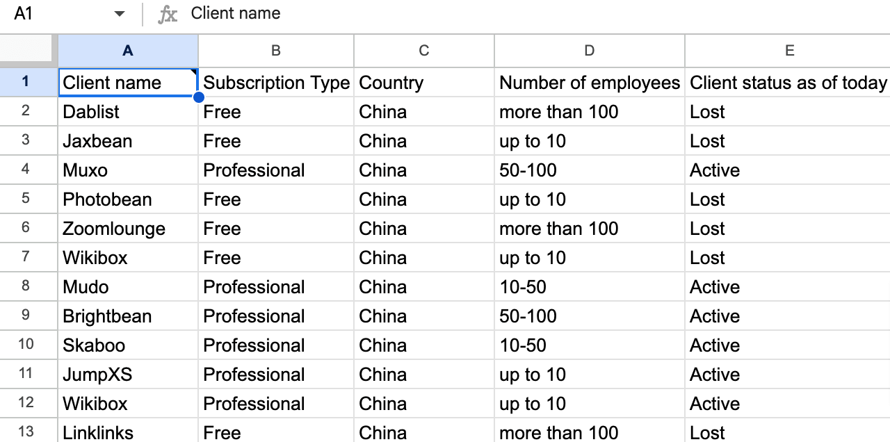
Here is a data set that we’ll use:
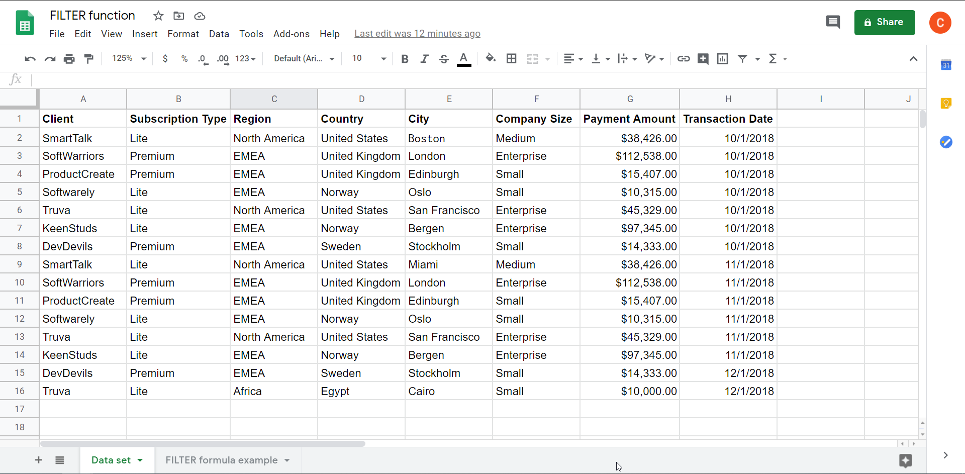
In this data set, we need to filter our clients that come from the EMEA (Europe, Middle East, and Africa) region only. Here is the formula to do this:
=filter('Data set'!A2:A,'Data set'!C2:C="EMEA")
'Data set'!A2:A– the Clients column to filter.'Data set'!C2:C="EMEA"– the filter condition: all"EMEA"values within the Region column.
This is the simplest FILTER formula example with only one condition. Meanwhile, you can filter out by multiple conditions, combine FILTER with other Google Sheets functions, and much more.
Google Sheets FILTER by multiple conditions (AND logic)
Note: Google Sheets FILTER function doesn’t support mixed conditions: the specified conditions can be for either columns or rows.
FILTER by the AND logic means that the formula will return the result if all the specified conditions are met.
Google Sheets FILTER by multiple conditions (AND logic) formula syntax
=FILTER(data_range,condition_1, condition_2, condition_3,...)
FILTER by multiple conditions (AND logic) Google Sheets formula example
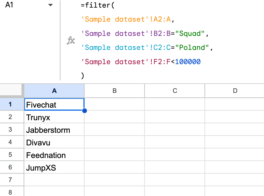
Let’s filter out clients ('Sample dataset'!A2:A) by the three conditions:
- Subscription type: Squad (
'Sample dataset'!B2:B="Squad") - Country: Poland (
'Sample dataset'!C2:C="Poland") - Payment amount: less than $100,000 (
'Sample dataset'!F2:F<100000)
Here is the formula:
=filter(
   'Sample dataset'!A2:A,
   'Sample dataset'!B2:B="Squad",
   'Sample dataset'!C2:C="Poland",
   'Sample dataset'!F2:F<100000
)
Link to the spreadsheet with the formula
Google Sheets FILTER by multiple conditions (OR logic)
FILTER with the OR logic means that FILTER will return the result if any or all of the specified conditions are met.
You can use FILTER with OR logic to specify multiple conditions from the same column.
FILTER by multiple conditions (OR logic) Google Sheets formula syntax
=FILTER(data_range,(condition_1.1)+(condition_1.2), condition_2,(condition_3.1)+(condition_3.2),...)
FILTER by multiple conditions (OR logic) Google Sheets formula example
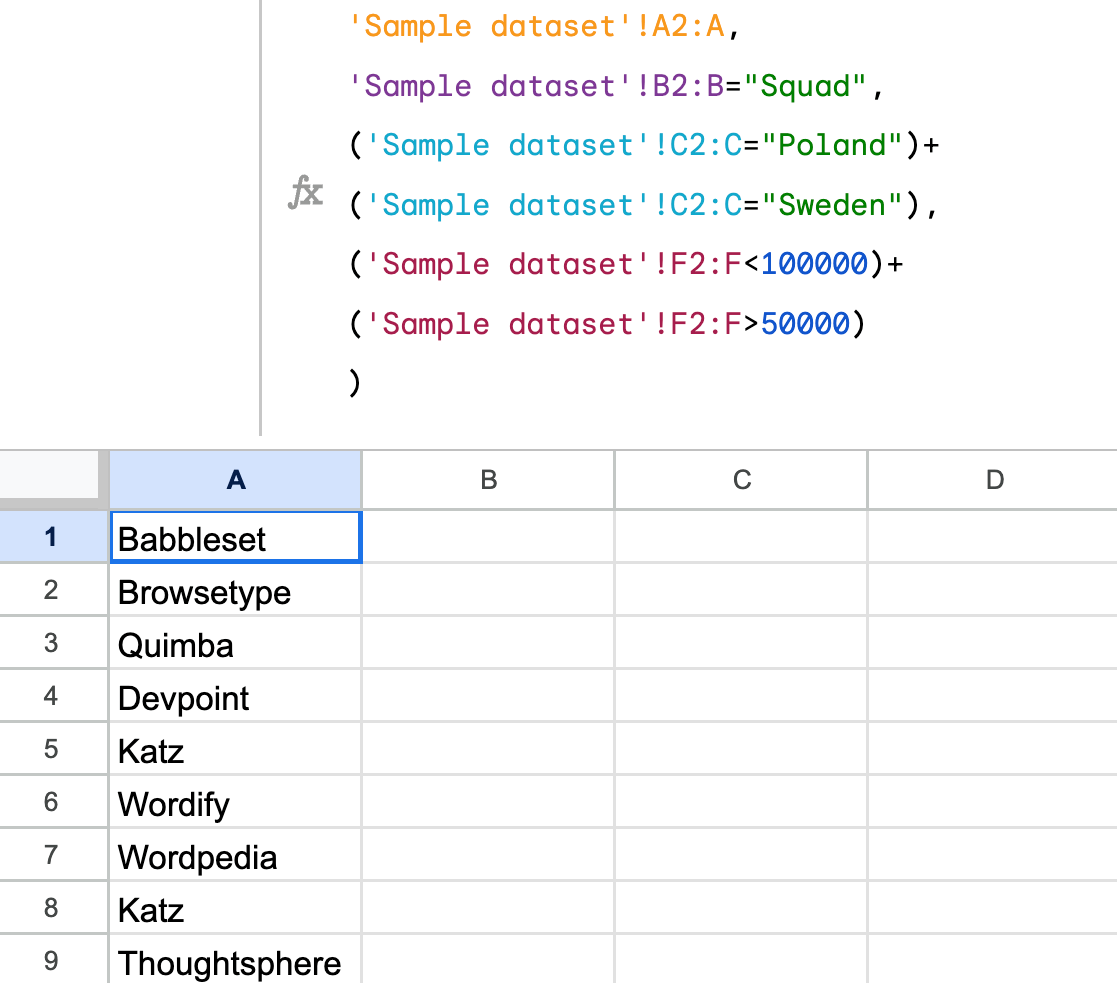
Let’s say you need to filter out clients ('Sample dataset'!A2:A) by different conditions from the same column:
- Subscription type: Squad (
'Sample dataset'!B2:B="Squad") - Country: Poland (
'Sample dataset'!C2:C="Poland") and/or Sweden ('Sample dataset'!C2:C="Sweden") - Payment amount: less than $100,000 (
'Sample dataset'!F2:F<100000) and/or more than $50,000 ('Sample dataset'!F2:F>50000)
Here is the formula:
=filter(
   'Sample dataset'!A2:A,
   'Sample dataset'!B2:B="Squad",
   ('Sample dataset'!C2:C="Poland")+
      ('Sample dataset'!C2:C="Sweden"),
   ('Sample dataset'!F2:F<100000)+
      ('Sample dataset'!F2:F>50000)
)
Link to the spreadsheet with the formula
Import data in Google Sheets and filter it without formulas
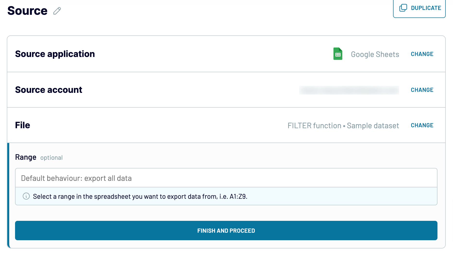
Now you know how to filter Google Sheets data with the FILTER function. But what if you first have to import data from another spreadsheet or an external source? It takes time to load data to your spreadsheet and then apply FILTER. However, you can use Coupler.io to filter data on the go without any formulas, importing it from 50+ sources.
Try this yourself with the form below. To get it started, select the data source and click Proceed. You can sign up with your Google account for free.
Let’s see how you can filter data from the abovementioned spreadsheet.
Choose FILTER function as the source file. Then specify your sheet – Sample dataset. Optionally, you can select a particular range you’d like to export.
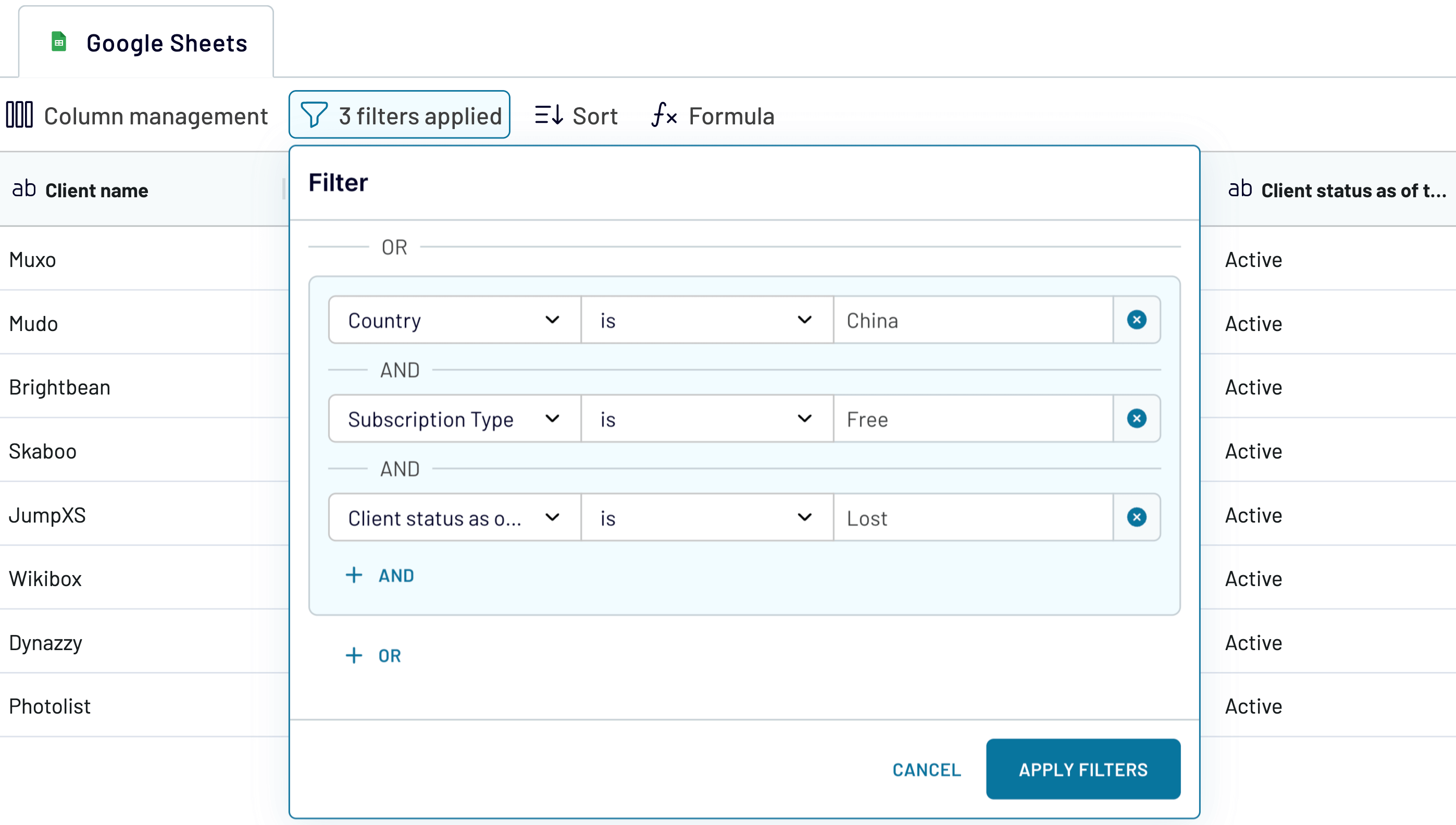
In the next step, you can filter your data by one or multiple criteria before loading your source data to the spreadsheet. For example, click Filter and then AND to filter out active clients from China with the Professional subscription:
- Select the column named Country, specify the condition “is”, then enter “China” as a value.
- Click +AND, select the column named Subscription Type, specify the condition “is”, then enter “Professional” as a value.
- Click +AND, select the column named Client Status, specify the condition “is”, then enter “Active” as a value.
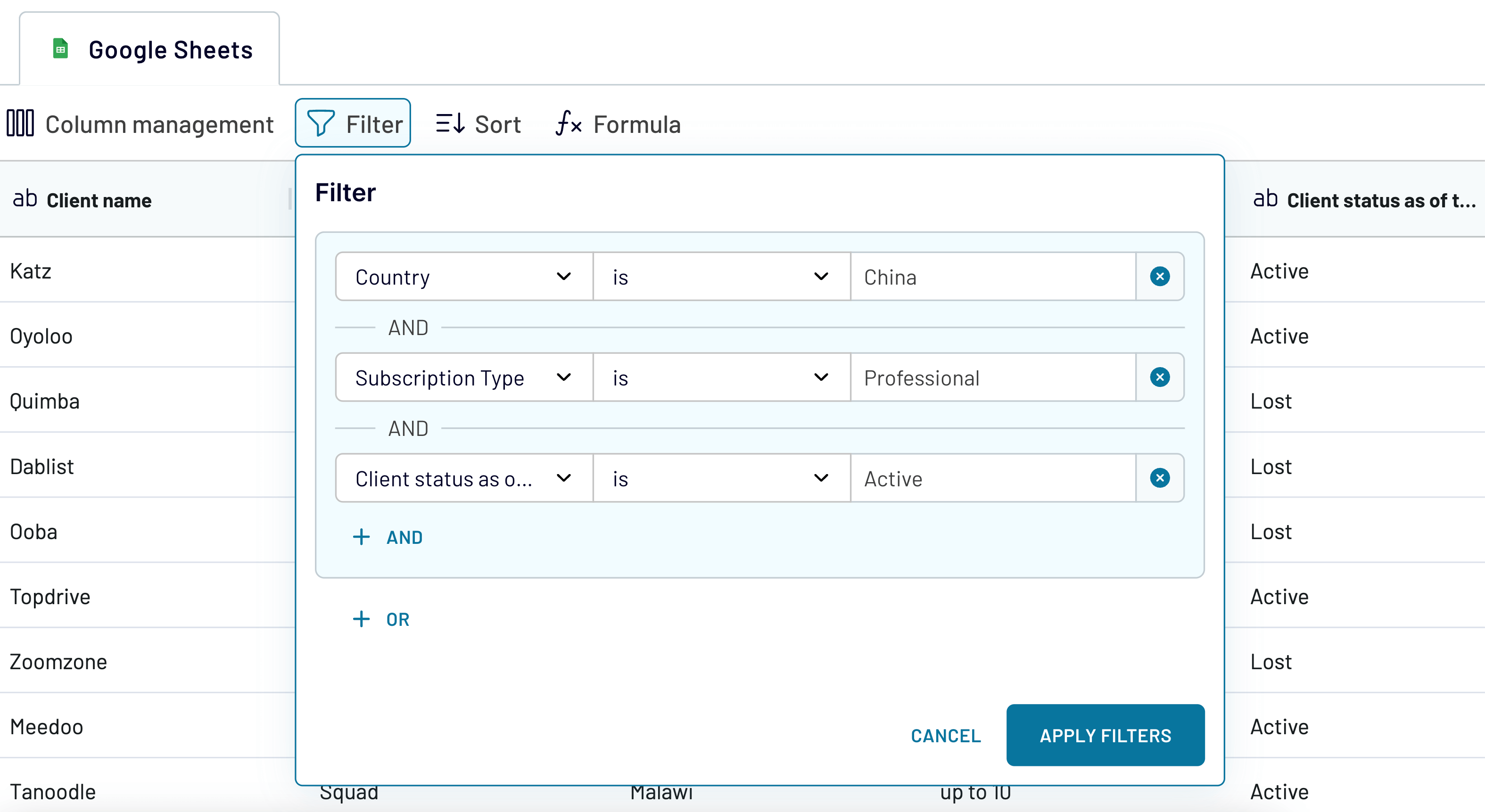
Let’s also filter out clients from China but this time with the Free subscription type and Lost status:
- Click OR.
- Select the column named Country, specify the condition “is”, then enter “China” as a value.
- Click +AND, select the column named Subscription Type, specify the condition “is”, then enter “Free” as a value.
- Click +AND, select the column named Client Status, specify the condition “is”, then enter “Lost” as a value.
- Click Apply filters.
Optionally, you can hide, add, and edit columns as well as sort data in ascending or descending order.
Once your data is transformed, proceed to the destination settings. You’ll need to choose the file and sheet where to import the queried data.
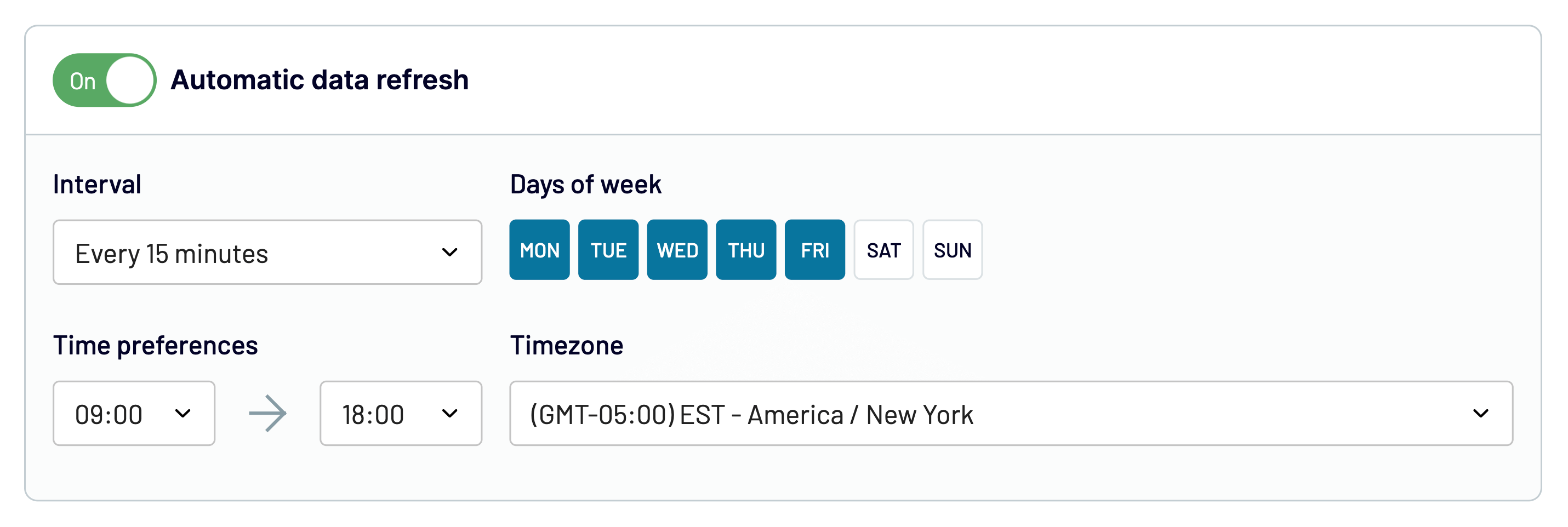
You can also select a schedule for data refresh to have your spreadsheet regularly updated. This way, you won’t miss out on any changes made to your source data.
Eventually, click Run importer. In a moment, you’ll have your data available in the destination spreadsheet:
With Coupler.io, you can save time, prevent human errors, and access the latest data you need.

Automate data export with Coupler.io
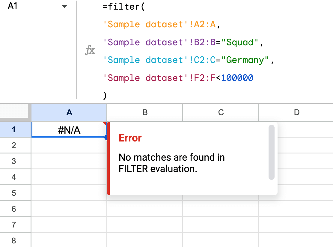
Get started for freeGoogle Sheets FILTER formula error: no matches are found in FILTER evaluation
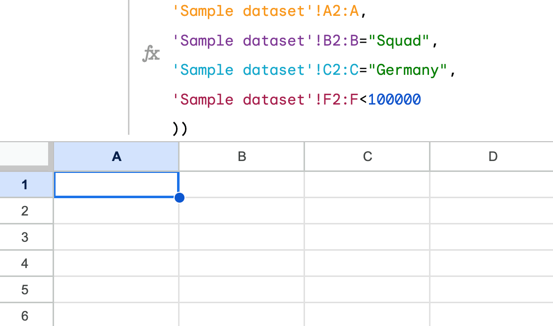
The FILTER No matches error occurs when there are no values that meet the specified conditions. For example, we know that we don’t have any clients from Germany with a payment amount below $100,000. So, the following formula will return #N/A:
=filter(
   'Sample dataset'!A2:A,
   'Sample dataset'!B2:B="Squad",
   'Sample dataset'!C2:C="Germany",
   'Sample dataset'!F2:F<100000
)
To make your FILTER formula return an empty cell instead of the #N/A error, add the IFERROR function at the beginning:
=iferror(
   filter(
      'Sample dataset'!A2:A,
      'Sample dataset'!B2:B="Squad",
      'Sample dataset'!C2:C="Germany",
      'Sample dataset'!F2:F<100000
   )
)
Link to the spreadsheet with the formula
FILTER by number in Google Sheets
Here are the conditions you can apply to filter numeric values:
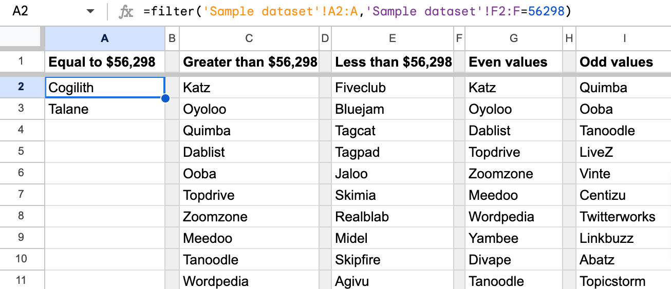
Google Sheets filter condition: Equal to X
Let’s filter out all clients with a payment amount equal to $56,298:
=filter('Sample dataset'!A2:A,'Sample dataset'!F2:F=56298)
Google Sheets FILTER condition: Greater than (“>”) X
Let’s filter out all clients with a payment amount greater than $56,298:
=filter('Sample dataset'!A2:A,'Sample dataset'!F2:F>56298)
Google Sheets FILTER condition: Less than (“<“) X
Let’s filter out all clients with a payment amount less than $56,298:
=filter('Sample dataset'!A2:A,'Sample dataset'!F2:F<56298)
Google Sheets FILTER condition: Not equal to X
Let’s filter out all clients with a payment amount not equal to $56,298:
=filter('Sample dataset'!A2:A,'Sample dataset'!F2:F<>56298)
Google Sheets FILTER condition: Even values
Let’s filter out all clients with even payment amounts:
=filter('Sample dataset'!A2:A,iseven('Sample dataset'!F2:F))
Google Sheets FILTER condition: Odd values
Let’s filter out all clients with odd payment amounts:
=filter('Sample dataset'!A2:A,isodd('Sample dataset'!F2:F))
Link to the spreadsheet with the formulas
FILTER by text in Google Sheets (exact match/non-match)
The basic filter by text includes two conditions:
- Return the values that are exactly equal to the specified text string
- Return the values that are exactly not equal to the specified text string
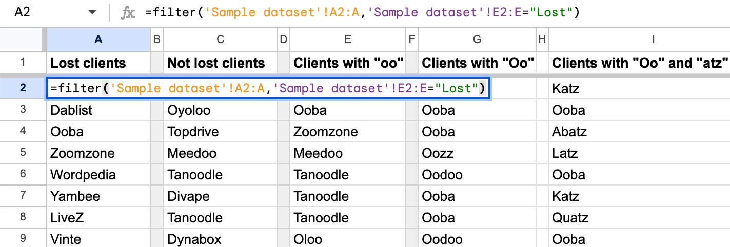
For example, let’s filter out clients with the lost status:
=filter('Sample dataset'!A2:A,'Sample dataset'!E2:E="Lost")
and those that have statuses other than lost:
=filter('Sample dataset'!A2:A,'Sample dataset'!E2:E<>"Lost")
Link to the spreadsheet with the formulas
Google Sheets FILTER by text (partial match)
In the blog post COUNTIF vs. COUNTIFS, we explained that you can use wildcards (“?” and “*“) to check the partial match of the data range. Wild cards do not work with FILTER. However, the SEARCH, FIND, and REGEXMATCH functions nested within the FILTER formula can do the job.
Use Google Sheets FILTER + SEARCH to filter by the needed text with the insensitive text case
SEARCH formula syntax
=SEARCH("text_to_search", cell_range, [starting_at])
text_to_search– the text you need to find.cell_range– the range to scan for the sought text.[starting_at]– the character number to start looking from (optional parameter).
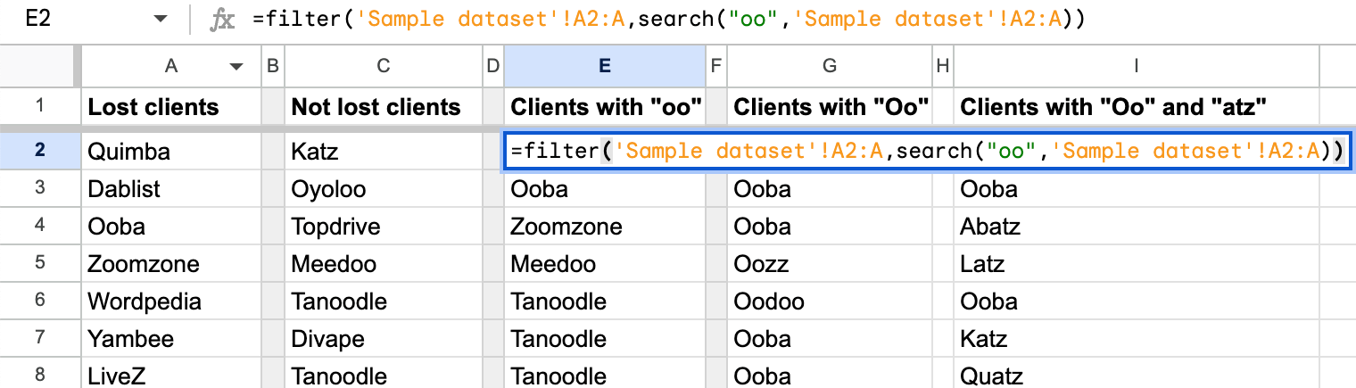
Now, let’s nest SEARCH within FILTER to filter out all clients with a double “o” (oo) in their names:
=filter('Sample dataset'!A2:A,search("oo",'Sample dataset'!A2:A))
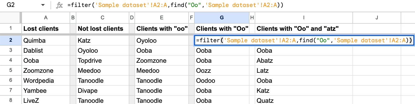
Use Google Sheets FILTER + FIND to filter by the needed text with the sensitive text case
If the text case matters for your filter criteria, nest the FIND function within the FILTER formula. FIND and SEARCH have the same formula syntax. So, let’s filter out all clients, who have “Oo” in their names.
=filter('Sample dataset'!A2:A,find("Oo",'Sample dataset'!A2:A))
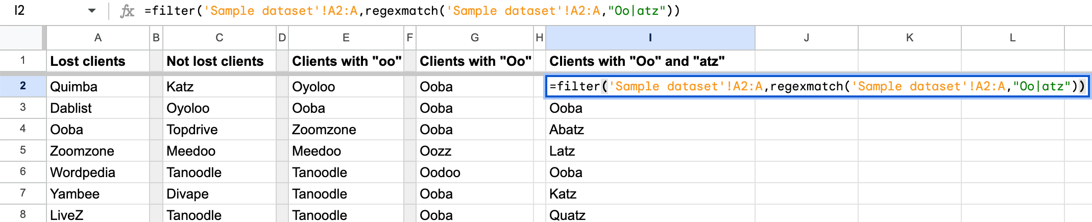
Use FILTER + REGEXMATCH for an advanced filter by text in Google Sheets
With REGEXMATCH, you can specify a regular expression to filter the data against. This function can replace both SEARCH and FIND, as well as provide additional filtering capabilities, such as filtering by multiple text conditions in the same column.
Google Sheets REGEXMATCH formula syntax
=REGEXMATCH(cell_range,"regular_expression")
cell_range– the range to scan for theregular_expressionregular_expression– the sequence of characters that define the text string to filter against.
For example, let’s filter out clients, who have “Oo” and “atz” in their names:
=filter('Sample dataset'!A2:A,regexmatch('Sample dataset'!A2:A,"Oo|atz"))
Link to the spreadsheet with the formulas
FILTER by date and time in Google Sheets
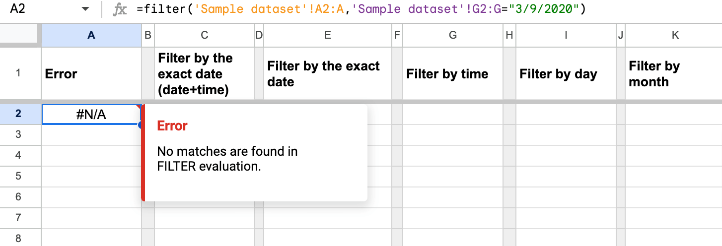
To filter values by date (full date, month, year, etc.), you’ll need to nest FILTER with additional functions.
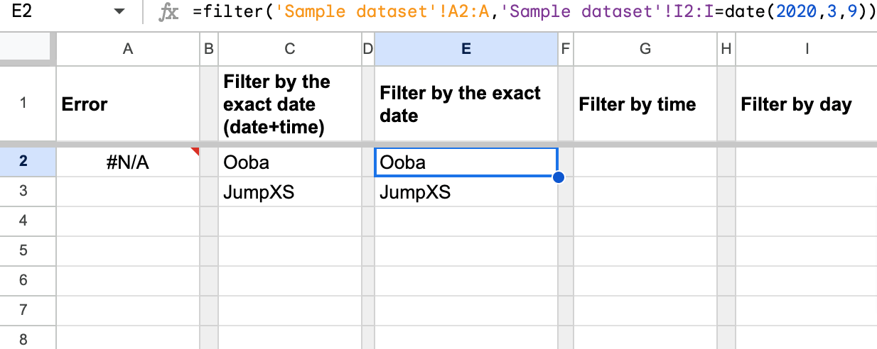
Note: if you simply try to use a date value as a text string in the filter criteria, you’ll get the No matches error:
=filter('Sample dataset'!A2:A,'Sample dataset'!G2:G="3/9/2020")
Let’s do this the right way.
Google Sheets filter by the exact date
Apply the DATE function within the FILTER formula as follows:
=FILTER(cell_range,cell_range=DATE(YYYY,MM,DD))
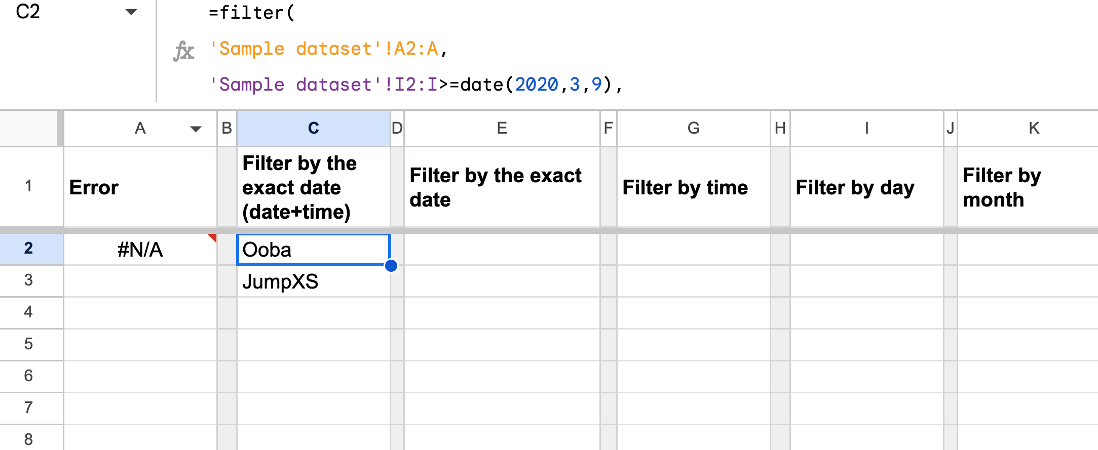
FILTER + DATE only works if your cell range doesn’t contain time units along with the date. If your date value looks like this: 3/9/2020 7:11:45, you’d better use the QUERY Google Sheets Function for filtering. With FILTER, your formula will be quite hefty and complex. For example, here’s how it looks when filtering out clients by the transaction date March 9, 2020:
=filter(
   'Sample dataset'!A2:A,
   'Sample dataset'!I2:I>=date(2020,3,9),
   'Sample dataset'!I2:I<date(2020,3,10)
)
In our data set, we have date+time values. Let’s split this column into two separate ones (for Date and Time), and check out how to filter these values. Here is the formula to use:
={"Date","Time"; arrayformula(split(G2:G," "))}
Read our dedicated blog post for more on how to split data in Google Sheets.
Now we can apply FILTER+DATE to filter out clients by the transaction date March 9, 2020:
=filter('Sample dataset'!A2:A,'Sample dataset'!I2:I=date(2020,3,9))
Use the comparison operators (“<” and “>”) to filter the results before or after the specified date.
Filter by time in Google Sheets
A similar syntax applies when you need to filter values by time:
=FILTER(cell_range,cell_range=TIME(HH,MM,SS))
For example, the formula to filter clients that performed the transaction before 10:46:23 is the following:
=filter(
   'Sample dataset'!A2:A,
   'Sample dataset'!J2:J<time(10,46,23)
)
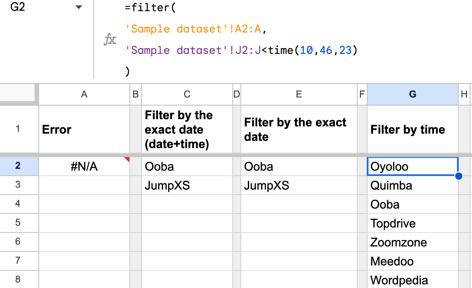
Use the comparison operators (“<” and “>”) to filter the results before or after the specified time.
Filter by day/month/year in Google Sheets
You can easily filter values by day/month/year using the respective functions (DAY, MONTH, and YEAR) and the following syntax:
=FILTER(cell_range,DAY(cell_range)=value)
For example, let’s filter out clients separately by:
- Day of month: 4
- Month: May
- Year: 2020
Here is how these filter criteria will look in the three separate FILTER formulas:
Day
=filter('Sample dataset'!A2:A,day('Sample dataset'!G2:G)=4)
Month
=filter('Sample dataset'!A2:A,month('Sample dataset'!G2:G)=5)
Year
=filter('Sample dataset'!A2:A,year('Sample dataset'!G2:G)=2020)
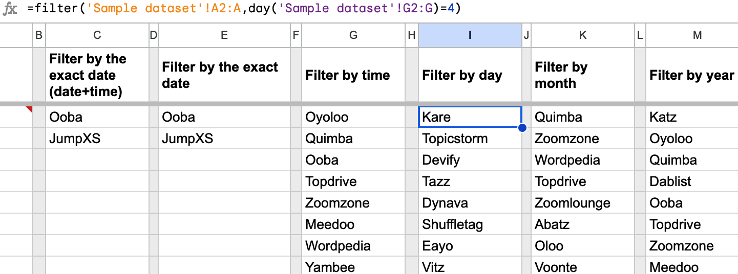
Use the comparison operators (“<” and “>”) to filter the results before or after the specified day/month/year.
Link to the spreadsheet with the formulas
Now, let’s explore some advanced case studies using the FILTER function.
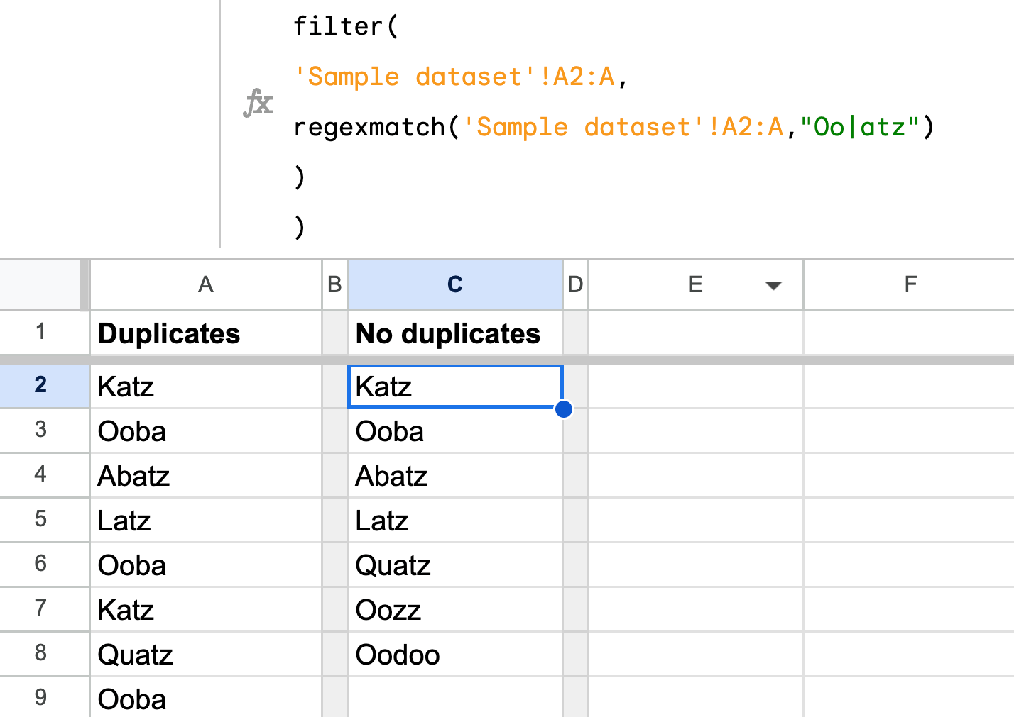
Remove duplicates in the filter results using FILTER+UNIQUE in Google Sheets
In the example with FILTER + REGEXMATCH, we’ve got many duplicates in the filter results. To remove duplicates, apply the UNIQUE function in your FILTER formula, as follows:
=unique(
   filter(
      'Sample dataset'!A2:A,
      regexmatch('Sample dataset'!A2:A,"Oo|atz")
   )
)
Link to the spreadsheet with the formula
Filter out duplicates in Google Sheets
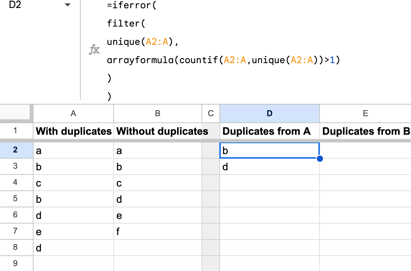
Let’s say you need to filter out duplicates (if any) of a cell range. Unfortunately, there is no NOT UNIQUE function in Google Sheets, which could have solved this task. But here is a workaround where you need to nest FILTER with UNIQUE, ARRAYFORMULA and COUNTIF:
=FILTER(
    UNIQUE(cell_range),
      ARRAYFORMULA(
         COUNTIF(cell_range,
            UNIQUE(cell_range))>1
      )
)
For example, there are two cell ranges: one with and one without duplicates. We applied the advanced FILTER formula to check both of them:
=iferror(
   filter(
      unique(A2:A),
         arrayformula(
            countif(A2:A,
               unique(A2:A))>1)
   )
)
and
=iferror(
   filter(
      unique(B2:B),
         arrayformula(
            countif(B2:B,
               unique(B2:B))>1)
   )
)
Link to the spreadsheet with the formulas
FILTER + IMPORTRANGE to filter the data imported from another Google spreadsheet
If you nest FILTER with IMPORTRANGE, you’ll be able to filter the data imported from another Google Sheets document. Here is the formula syntax:
=FILTER(IMPORTRANGE("spreadsheet", "cell_range"),[condition_1, condition_2,...])
spreadsheet– the URL or ID of the spreadsheet to import data from.cell_range– a range of cells to query.condition– a range that contains the filter criteria.
Read our Google IMPORTRANGE Tutorial to check out the formula example and learn more about how to use IMPORTRANGE.
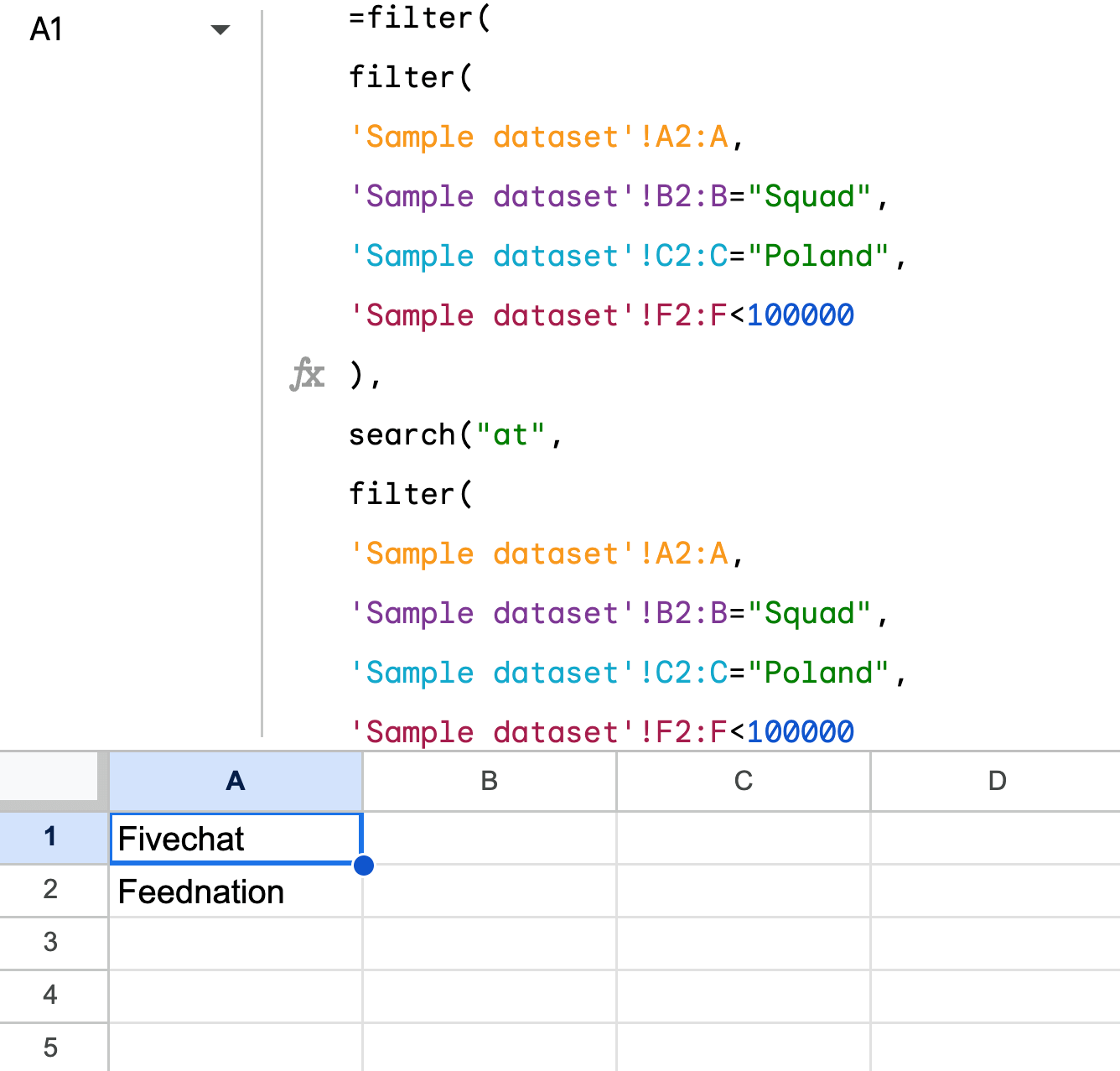
FILTER + FILTER to filter the filtered results in Google Sheets
FILTER + FILTER Google Sheets formula syntax
=FILTER(FILTER(cell_range, condition),condition)
This combination lets you filter a result that has already been filtered. This sounds complicated, but here is an example. We want to filter clients by the three conditions:
- Subscription type: Squad
- Country: Poland
- Payment amount: less than $100,000
The filter result should be filtered by partial text match “at“. Here is how the formula looks:
=filter(
   filter(
      'Sample dataset'!A2:A,
      'Sample dataset'!B2:B="Squad",
      'Sample dataset'!C2:C="Poland",
      'Sample dataset'!F2:F<100000
   ),
   search("at",
      filter(
         'Sample dataset'!A2:A,
         'Sample dataset'!B2:B="Squad",
         'Sample dataset'!C2:C="Poland",
         'Sample dataset'!F2:F<100000
      )
   )
)
Link to the spreadsheet with the formula
FILTER + LARGE Google Sheets to filter the top X records
FILTER + LARGE Google Sheets formula syntax
=FILTER(cell_range,criteria_range>=LARGE(criteria_range,rank))
Let’s filter out the top 5 clients by the payment amount. Here is the formula:
=filter(
   'Sample dataset'!A2:A,
   'Sample dataset'!F2:F>=large('Sample dataset'!F2:F,5)
)
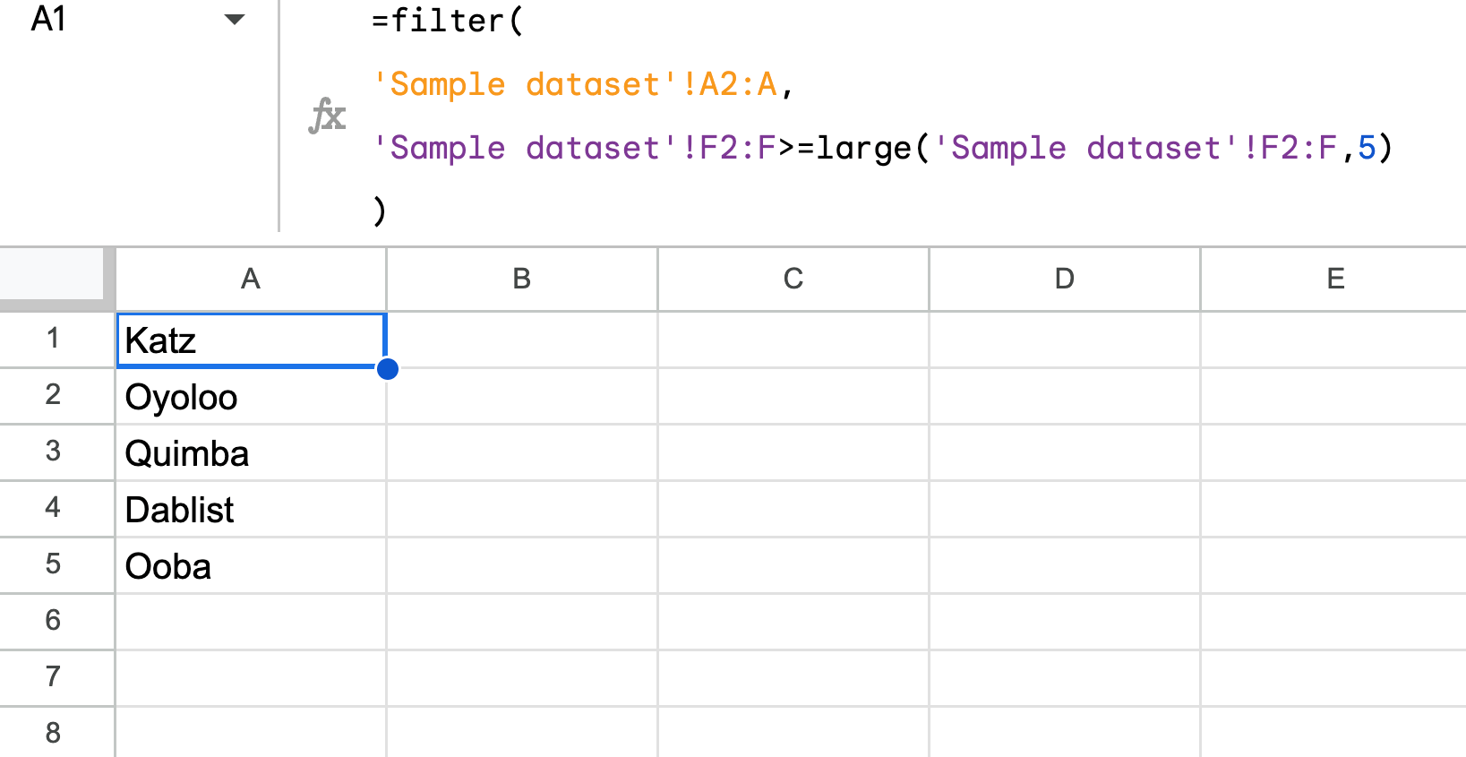
If you need to filter by the smallest values instead of largest, use the SMALL function instead of LARGE.
Link to the spreadsheet with the formula
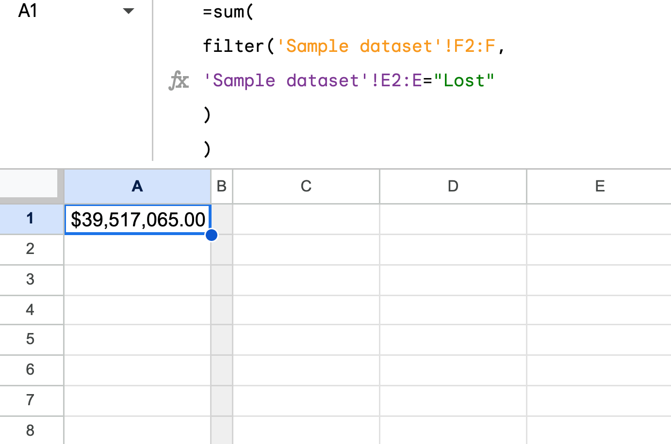
SUM + FILTER to sum the filtered results in Google Sheets
If you combine FILTER with SUM, the formula will return the sum of the filtered results. Here is the syntax:
=SUM(FILTER(cell_range, condition))
For example, here is the formula to sum the payment amount of all lost clients:
=sum(
   filter('Sample dataset'!F2:F,
   'Sample dataset'!E2:E="Lost"
   )
)
Filter data and add a total row below
Let’s say we want to do the following:
- Filter clients by two conditions: “lost” status and transaction date after Jul 1, 2020
- Retrieve specific columns (Client Name, Subscription Type, Country, and Payment Amount)
- Calculate the total payment amount of the lost clients
- Place the total sum in a separate row below the filter results
Let’s go step-by-step to see how the advanced FILTER formula can do this:
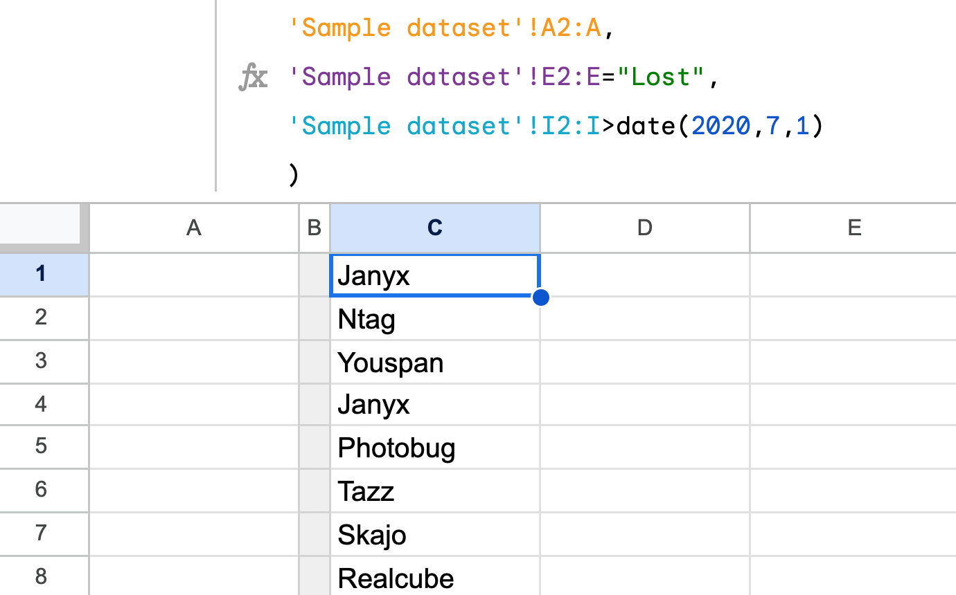
Filter clients by two conditions: “lost” status and transaction date after Jul 1, 2020
=filter(
   'Sample dataset'!A2:A,
   'Sample dataset'!E2:E="Lost",
   'Sample dataset'!I2:I>date(2020,7,1)
)
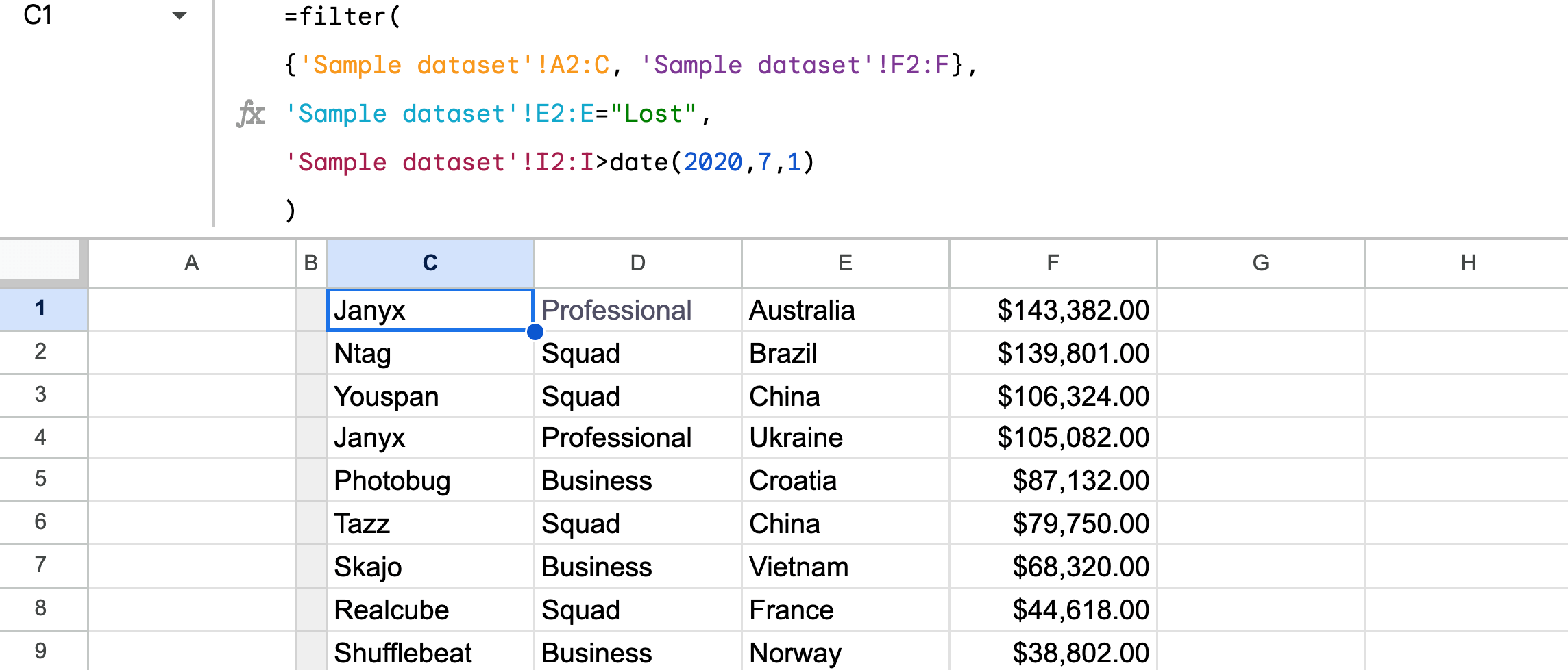
Retrieve specific columns (Client Name, Subscription Type, Country, and Payment Amount)
=filter(
   {'Sample dataset'!A2:C, 'Sample dataset'!F2:F},
   'Sample dataset'!E2:E="Lost",
   'Sample dataset'!I2:I>date(2020,7,1)
)
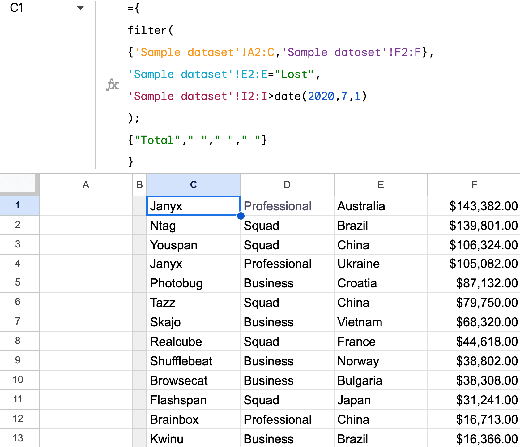
Place a separate row for total sum below the filter results
={
   filter(
      {'Sample dataset'!A2:C,'Sample dataset'!F2:F},
      'Sample dataset'!E2:E="Lost",
      'Sample dataset'!I2:I>date(2020,7,1)
   );
   {"Total"," "," "," "}
}
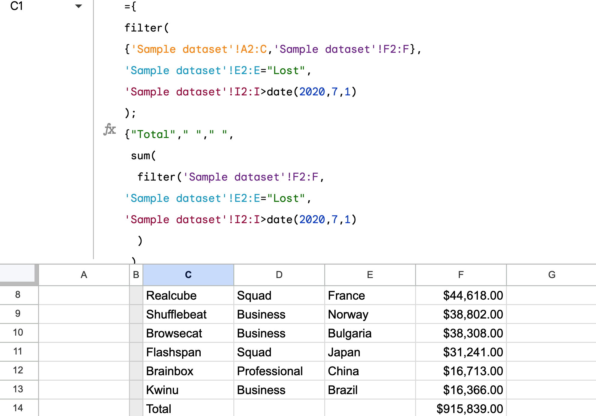
Calculate the total payment amount of the filtered clients
={
   filter(
      {'Sample dataset'!A2:C,'Sample dataset'!F2:F},
      'Sample dataset'!E2:E="Lost",
      'Sample dataset'!I2:I>date(2020,7,1)
   );
   {"Total"," "," ",
       sum(
        filter('Sample dataset'!F2:F,
         'Sample dataset'!E2:E="Lost",
         'Sample dataset'!I2:I>date(2020,7,1)
       )
      )
   }
}
Link to the spreadsheet with the formula
This is a rather tricky FILTER formula. Watch this YouTube video to learn more advanced tricks with FILTER and other Google Sheets functions.
FILTER is an awesome Google Sheets function, isn’t it?
FILTER is a very flexible and popular Google Sheets function. Besides, it is one of the most frequently used functions in the cases covered in our blog. It was used to build a sales tracker, as well as explain other Google Sheets functions, such as IFS vs. nested IF statements.
For data from other spreadsheets or external sources, use Coupler.io to import and filter it on the go without any formulas. Get started for free to check it out by yourself!
Automate data export with Coupler.io
Get started for free