There comes a time in the life of every Google Sheets user when you need to reference a certain data range from another sheet, or even a spreadsheet, to create a combined master view of both. This will let you consolidate information from multiple worksheets into a single one.
Another frequent case may raise a requirement for a backup spreadsheet that would be copying values and format from the source file, but not the formulas. Some of the users may also want their master document to update automatically, on a set schedule.
So, if you are struggling to find the solution to the above tasks, keep reading this article. You’ll find tips on how to link data from other sheets and spreadsheets, as well as discover alternative ways of doing so. In the end, I will provide a full comparison of the approaches mentioned for you to be able to evaluate and choose from.
How to reference data from other sheets or tabs – what are the options?
There are multiple cases and ways to reference data in Google Sheets. You can reference another sheet in Google Sheets, a cell or a cell range, as well as columns and rows. In addition, you may need to import data from one sheet/spreadsheet to another based on certain criteria or even combine data from multiple sheets into one view.
Google Sheets offers a few native options for data referencing including the IMPORTRANGE function. However, you should keep in mind that
Google Sheets native functions and options only allow you to reference data not import it.
Yes, Google Sheets does not provide a functionality that actually imports data from one sheet/spreadsheet to another although the name of the IMPORTRANGE function suggests the opposite. They only reference a specified range, i.e., if the data in your source sheet is not available, you won’t have access to it in your destination sheet. This is a drawback. So, if you need to import data (range of cells, columns, or rows) from one sheet to another, you’ll need to opt for a third-party solution, either a web app or Google Sheets add-on. Or, you can simply copy data from another sheet in Google Sheets, but it’s more for noobies 🙂
Below, we cover both native Google Sheets options to reference data and third-party tools to import data between Google Sheets. Let’s start with the native ones.
If Excel spreadsheets are in your focus, then head on to our blog post about how to link sheets in Excel.
#1 – How to link sheets in Google Sheets using FILTER function
You can use formulas for referencing columns or rows to link cell ranges between different sheets of the same spreadsheet. We’ll talk about this later in this section. First, let’s start with more advanced cases to link sheets using the FILTER function in Google Sheets.
Google Sheets link to another sheet based on criteria
Let’s say, you want to filter your data set by specific criteria and import the filtered values into another sheet. You can do this using the FILTER function that was featured in the example above. Here is the syntax:
=FILTER(data_set,criterium1, criterium2,...)data_set– a range of cells to filter.criterium– the criteria to filter the data set.
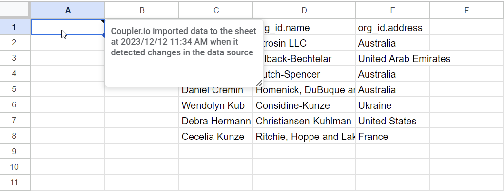
As an example, we’re going to filter users by country, Australia, and import the results into another sheet.
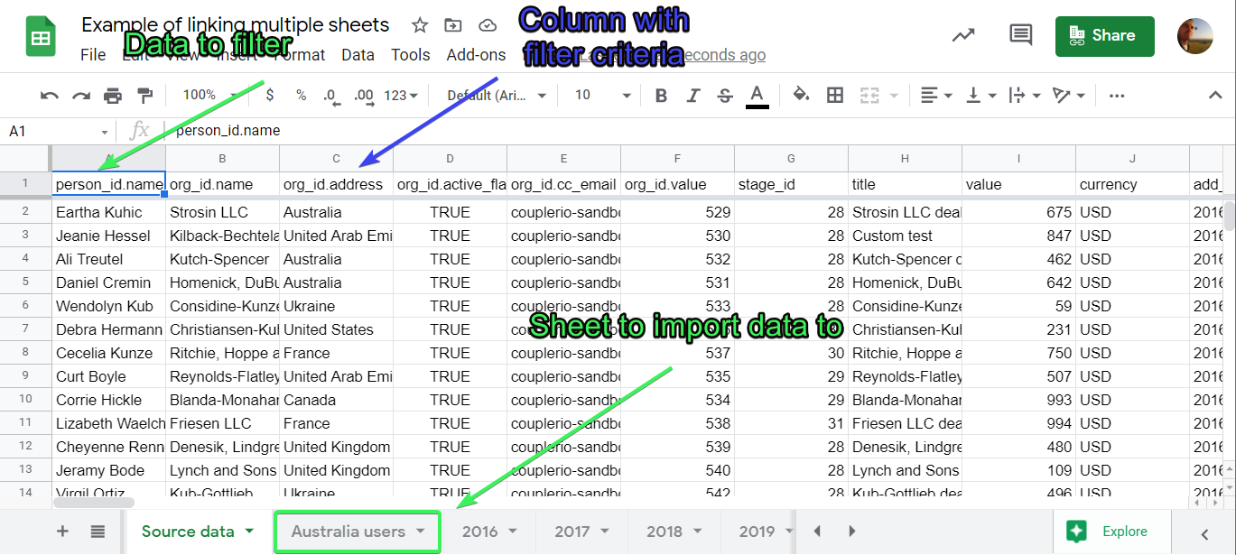
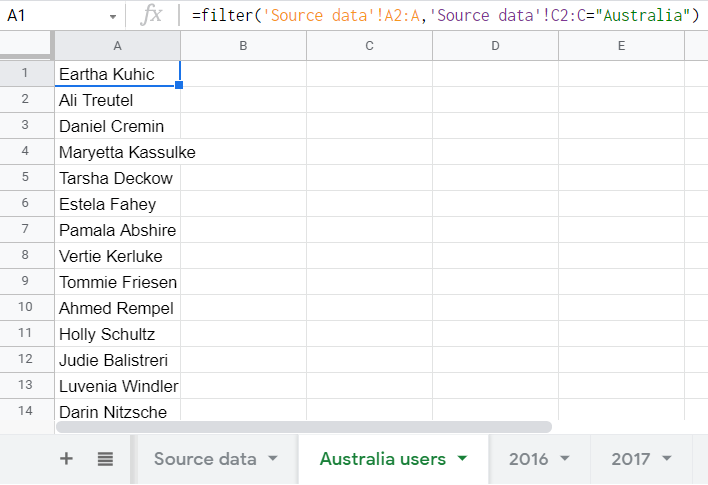
Here is what our formula will look like:
=filter('Source data'!A2:A,'Source data'!C2:C="Australia")
Read about the Google Sheets FILTER function to discover more filtering options.
How to import data from multiple sheets into one column
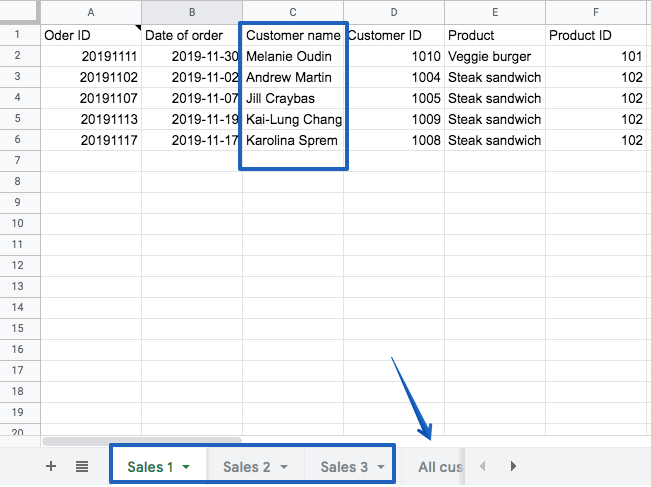
Let’s review an example of when one needs to link data from several columns in different sheets into one.
In my example, I have three different tabs with sales data: Sales 1, Sales 2, and Sales 3. My task is to collect all customer names in the sheet called All customers.
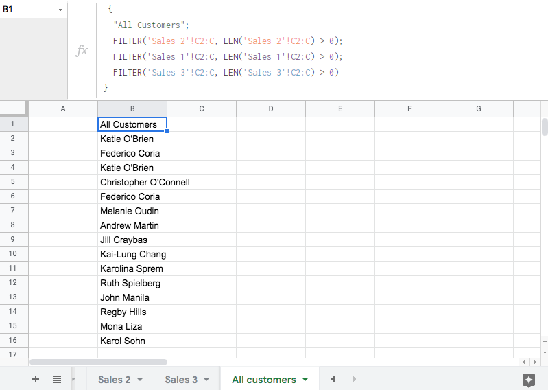
To do it, I’ll use this formula:
={
  "All Customers";
  FILTER('Sales 2'!C2:C, LEN('Sales 2'!C2:C) > 0);
  FILTER('Sales 1'!C2:C, LEN('Sales 1'!C2:C) > 0);
  FILTER('Sales 3'!C2:C, LEN('Sales 3'!C2:C) > 0)
}
Where:
"All Customers"– is a given name of my column,FILTER('Sales 1'!C2:C, LEN('Sales 1'!C2:C)> 0)– this expression means that I take all data from column C of “Sales 1”, excluding the values that are equal to or less than 0.
As a result, I get the names of all my customers from three different sheets gathered in one column.
One of the advantages of this approach is that I can change the names of my data source sheets (where I take data from), and they will automatically be updated in the formula!
See how it works:

At the same time, there is a better option to consolidate your data from multiple Google Sheets into one master view – we’ve covered it in this section.
#2 – How to reference another spreadsheet/workbook in Google Sheets via IMPORTRANGE
The options introduced above work for referencing data between sheets of a single Google Sheets document. If you need to link to another spreadsheet (sheet or tab of a different Google Sheets document), then you need IMPORTRANGE. It’s a Google Sheets function that allows you to import a data range from one spreadsheet to another. However, it does not actually import data but only references it.
To reference another sheet in a Google Sheets spreadsheet, follow these instructions:
- Go to the spreadsheet you want to export data from. Copy its URL.
- Open the sheet you want to upload data to.
- Place your cursor in the cell where you want your imported data to appear.
- Use the syntax as described below:
=IMPORTRANGE("spreadsheet_url", "range_string")
Where spreadsheet_url is a Google Sheets link to another sheet, which you copied earlier where you want to pull the information from.
range_string is an argument that you put in quotes to define what sheet and range to upload data from.
For example:
- Use
"new students!B2:C"to name the sheet and range to get information from. - Use
"A1:C10"to state a range of cells only. In this case, if you don’t define the sheet to import from, the default behavior is to upload data from the first sheet in your spreadsheet.
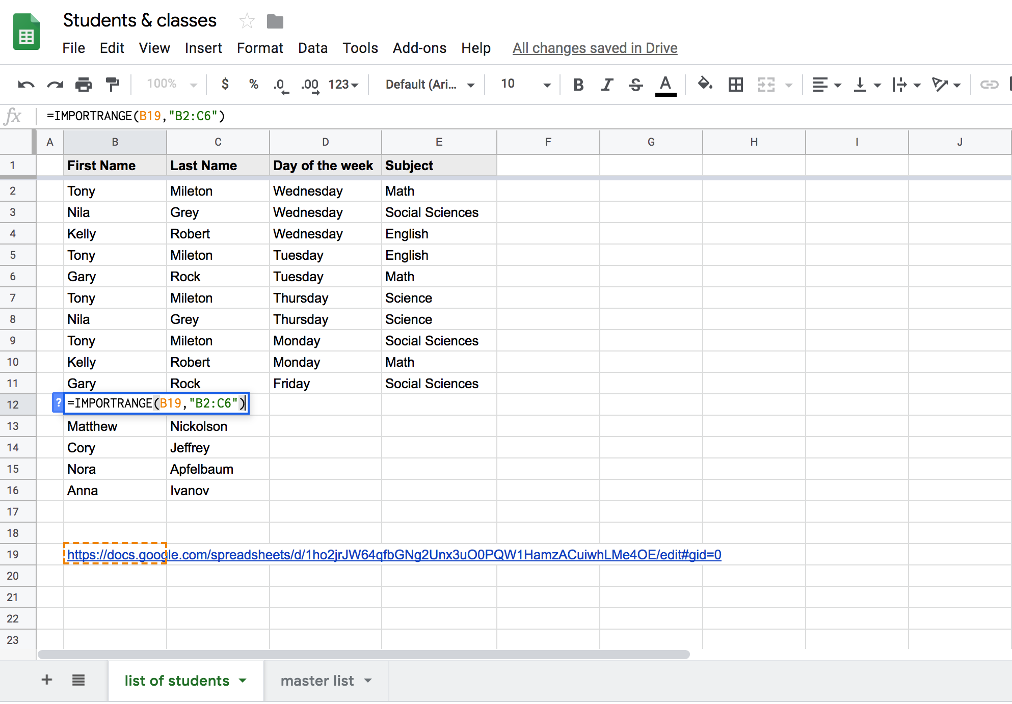
You may also use
=IMPORTRANGE(B19, "B2:C6")
if B19, in this case, entails the necessary spreadsheet URL to link data from.
Note: the use of IMPORTRANGE anticipates that your destination spreadsheet must get permission to pull data from another document (the source). Every time you want to import information from a new source, you will be required to allow this action to happen. After you provide access, anybody with edit rights in your destination spreadsheet will be able to use IMPORTRANGE to import data from the source. The access will be valid for the time the person who provided it is present in the data source. For more about this Google Sheets function, read our IMPORTRANGE Tutorial.
In my case, my formula looks like this :
=IMPORTRANGE("spreadsheet_url","new students!B2:C")
Or
=IMPORTRANGE("spreadsheet_url","B2:C")
because new students is the only sheet I have in my spreadsheet.
However, the IMPORTRANGE solution has several drawbacks. The one I would mention relates to a negative impact on the overall spreadsheet performance. You can google IMPORTRANGE in the Google Community forum to see a number of threads that explain the issue in more detail. Basically, the more IMPORTRANGE formulas you have in your worksheet, the slower the overall productivity will be. The spreadsheet will either stop working or require a lot of time to process and therefore display your data.
How to link two Google Sheets without the IMPORTRANGE function
While using IMPORTRANGE is one of the most common methods to link two different Google Sheets, there are some other options as well:
- Google Sheets API. This is an advanced method that is not suitable for most users as it requires programming skills to connect one spreadsheet to another. However, using this method is also possible. Luckily, the other two methods on our list are suitable for people without any tech background.
- Data integration solutions. These are specialized tools that can automatically connect various apps and automate data flows. It’s also possible to use them to link two Google Sheets. Coupler.io is one of those, which is also available as an add-on. I recommend trying it as it’s very easy to use. I’ll explain how to link two different Google Sheets with Coupler.io in the next section.
- Third-party add-ons. There are various add-ons available in the Google Workspace Marketplace that can help you expand the native functionality. For example, Coupler.io and Sheetgo allow you to link two Google Sheets without any formulas. For this reason, they are even called an “Importrange alternative”.
#3 – How to pull data from another sheet in Google Sheets without formulas
There is no native way to import data from one sheet or spreadsheet to another in Google Sheets. You can do this job with Coupler.io.
How to import data from another Google sheet or spreadsheet with Coupler.io
Click Proceed in the form below, where we already selected Google Sheets as both source and destination.
You can sign up for free with your Google account. Then complete the following steps to set up the integration.
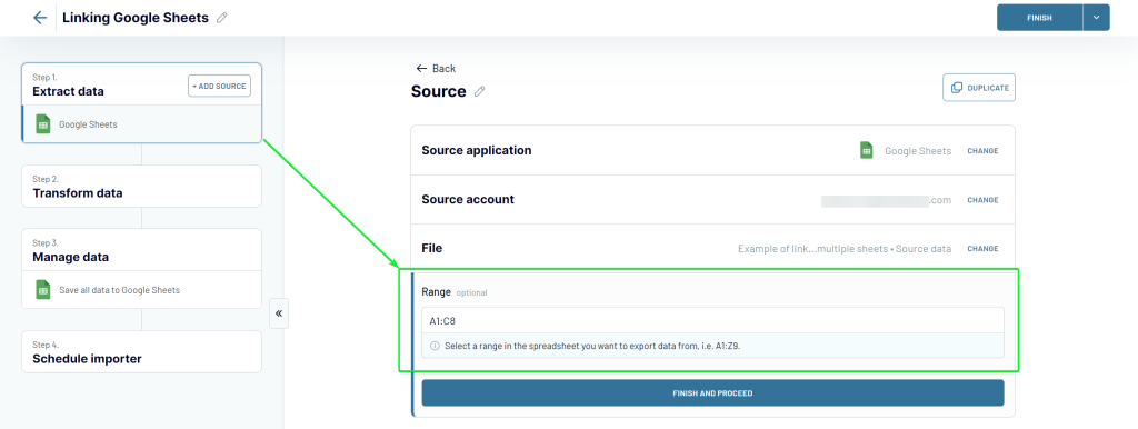
Step 1. Extract data from a source sheet
- Connect to your Google account.
- On your Google Drive, select a spreadsheet and a sheet to import data from. You can select multiple sheets if you want to merge data from them into one master view.
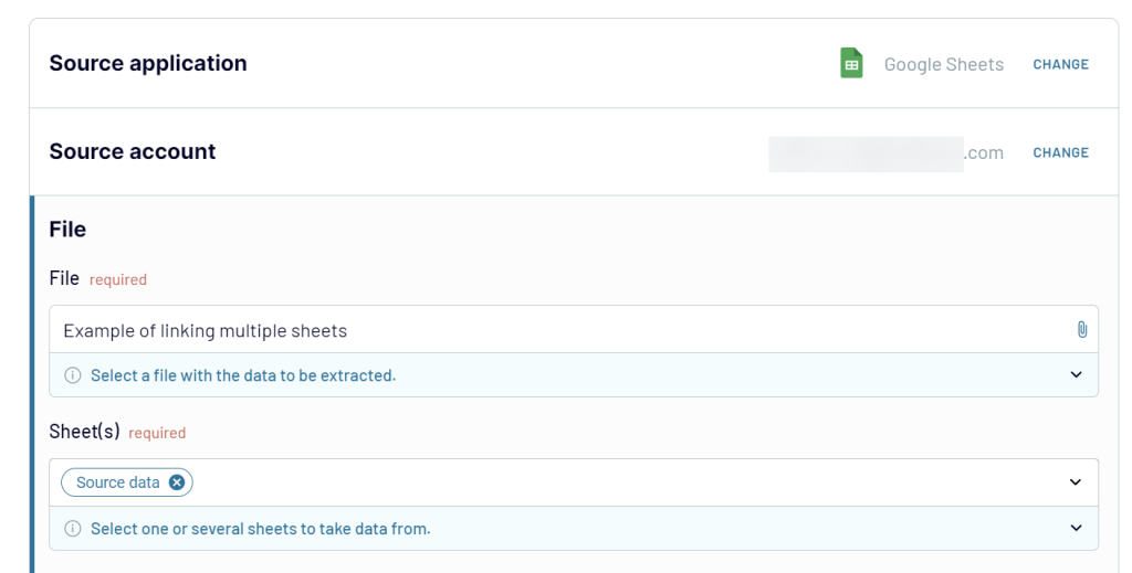
Optionally, you specify a range to export data from, for example, A1:Z9, if you don’t need to pull data from an entire sheet.
Coupler.io allows you to load data from multiple sheets of a single spreadsheet. If you want to combine data from multiple spreadsheets, then you can click Add one more source and connect one more spreadsheet to import data from.
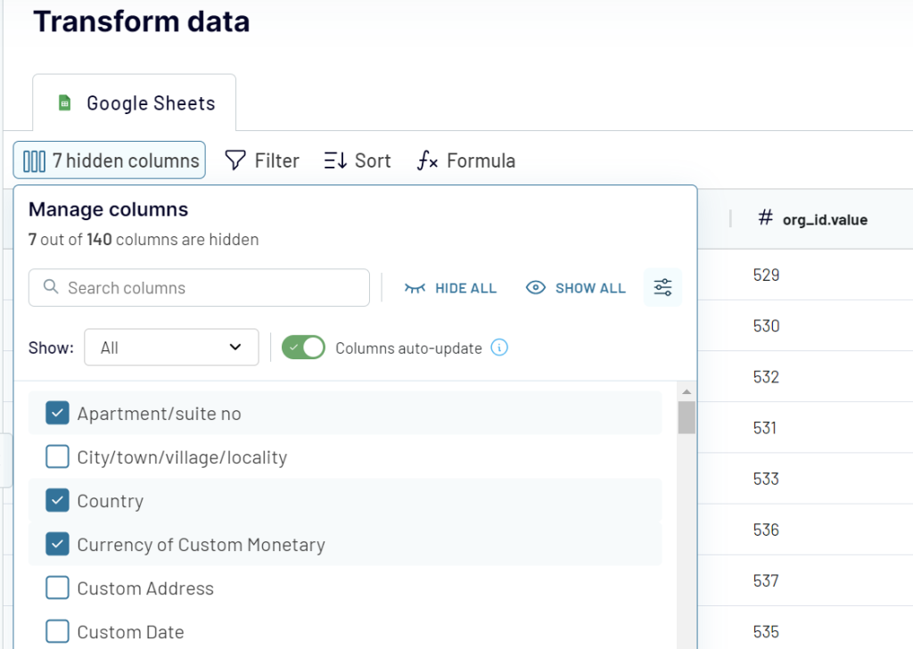
Step 2. Transform data
At the next step, you can preview and even transform the data to import. Coupler.io allows you to:
- Hide/unhide columns, edit column names and their types.
- Filter and sort data
- Create new columns using supported formulas.
Step 3. Manage data to load to a destination sheet
- Connect to your Google account.
- Select a file on your Google Drive and a sheet to load data to, You can create a new sheet by entering a new name.
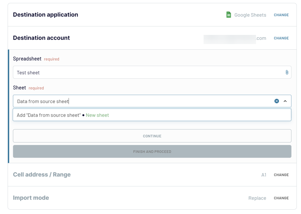
Optionally, you can change the first cell where to import your data range (A1 cell is set by default) and change the import mode for your data: replace your previous information or append new rows under the last imported entries. You can also toggle on the Last updated column feature if you want to add a column to the spreadsheet with the information about the last date and time refresh.
Once this step is complete, you can run the import right away and link your Google Sheet to another sheet. If you want to automate data import on a schedule, see the instructions in the next section.
How to sync two Google Sheets on a schedule without formulas using Coupler.io
Coupler.io allows you to easily sync two Google Sheets on a custom schedule. Once you complete the steps described above and your Coupler.io importer is almost ready, you can specify your preferences for the data refresh. Toggle on the Automatic data refresh and customize the schedule.
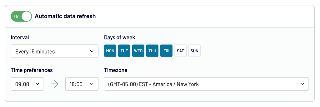
In the end, click Run importer to sync two Google Sheets. Now, the latest information from the source spreadsheet will be automatically transferred to the destination sheet during the next scheduled update.
By the way, you can also use Coupler.io as a Google Sheets add-on. Watch our YouTube video on how to install the Coupler.io add-in and set up a Google Sheets importer.
How to reference cell in another workbook in Google Sheets with Coupler.io
Coupler.io allows you to not only reference another workbook in Google Sheets but also import an exact cell range that only fits into the specified range. For example, you want to pull data from the range A1:C8 of one workbook and insert it into the range C1:E8 of another workbook. For this, perform the setup as described above, but also specify the following parameters:
- Range of the source spreadsheet (Step 1) – here you’ll need to specify the range of cells to import data from. In our example, A1:C8
- Cell address / Range of the destination spreadsheet (Step 3) – here you’ll need to specify the range of cells to import data to. In our example, C1:E8
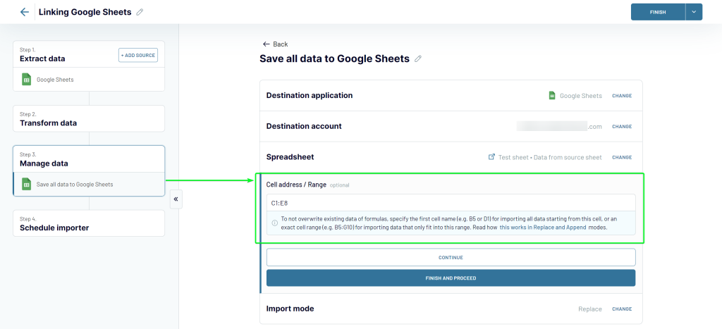
Click Save and Run and welcome your data in the specified range of cells.
Importing data is not the only thing you can do with Coupler.io. This reporting automation solution also allows you to consolidate or stitch data from different Google Sheets and even sources. Let’s check out a simple example below.

Automate data export with Coupler.io
Get started for free#4 – Pull data from multiple sheets of a single Google Sheets doc
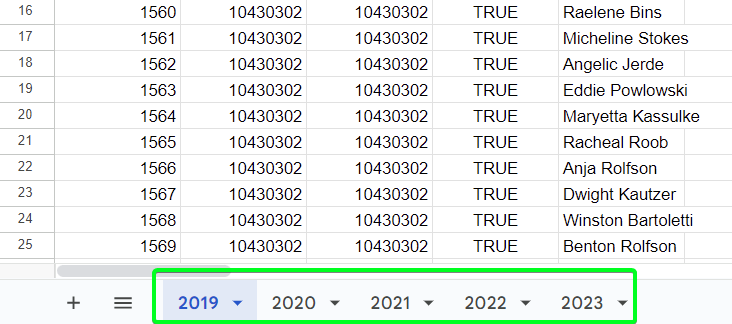
We have a Google Sheets doc with five sheets that contain data about deals for different years: 2019, 2020, 2021, 2022, and 2023:
Instead of manually copying data from each sheet or building a complex IMPORTRANGE formula, we can simply list all these sheets when setting up a Google Sheets importer as follows:
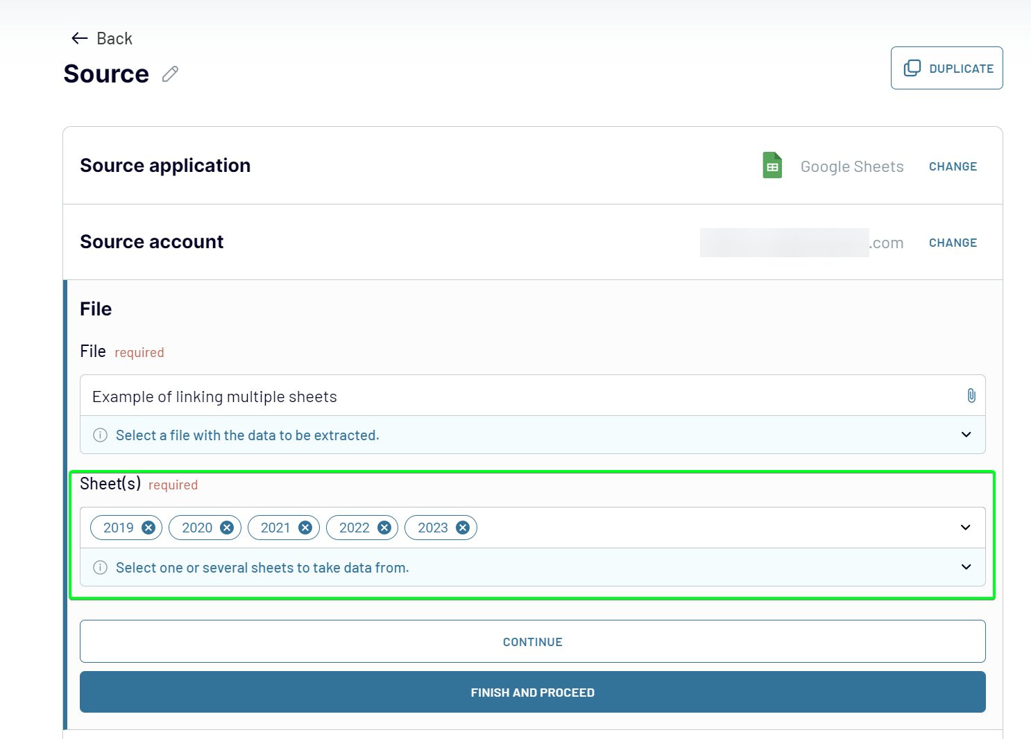
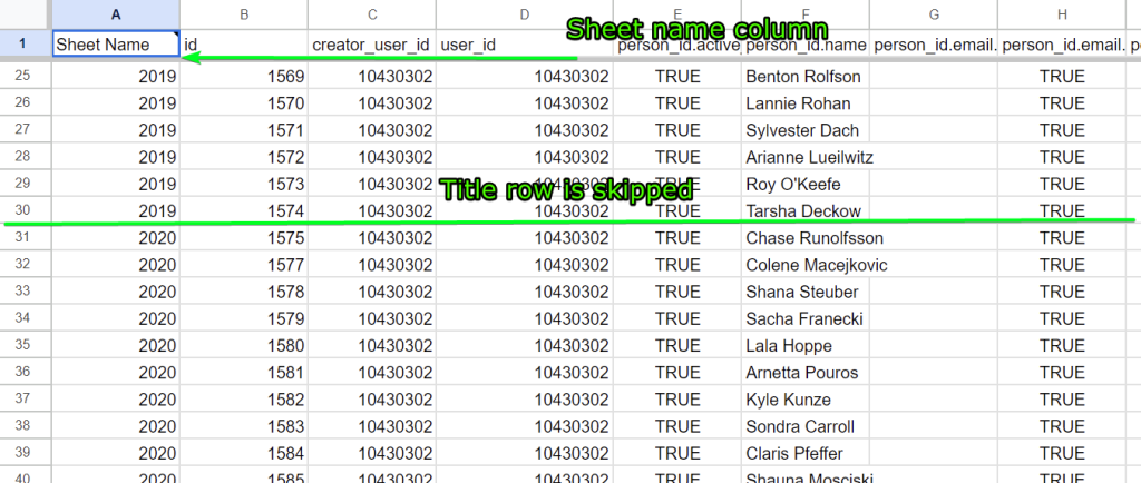
Click Save and Run and the data from the sheets will be pulled into our destination sheet. What are the main benefits? You’ll get a column indicating which sheet a data set belongs to. Besides, the title rows from each sheet except for the first one are skipped, so you get a smooth merge of data.
If you want to do the same using IMPORTRANGE, here is what your formula should look like:
={IMPORTRANGE("1XTBc1P49IPqZoWQldeOphvU2fa5gguBSW6poS8x5rW8","2019!A1:EU30");
IMPORTRANGE("1XTBc1P49IPqZoWQldeOphvU2fa5gguBSW6poS8x5rW8","2020!A2:EU572");
IMPORTRANGE("1XTBc1P49IPqZoWQldeOphvU2fa5gguBSW6poS8x5rW8","2021!A2:EU972");
IMPORTRANGE("1XTBc1P49IPqZoWQldeOphvU2fa5gguBSW6poS8x5rW8","2021!A2:EU1243");
IMPORTRANGE("1XTBc1P49IPqZoWQldeOphvU2fa5gguBSW6poS8x5rW8","2023!A2:EU204")}
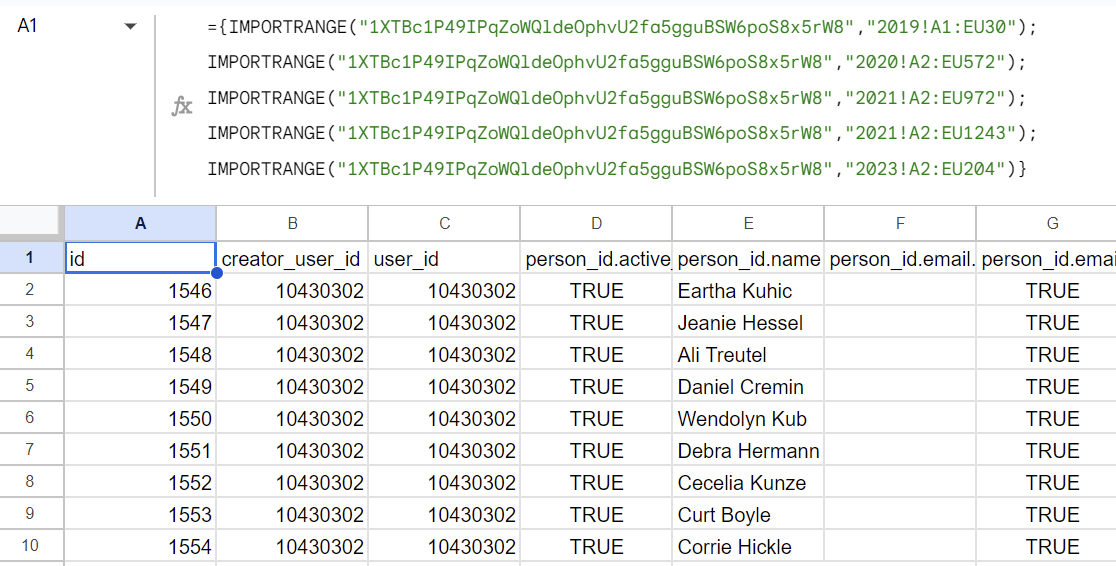
It’s important to specify exact data ranges like 2020!A2:EU972, otherwise, you’ll get multiple blank rows between the data. And do not expect to get your data right away – IMPORTRANGE works pretty long. In our case, we had to wait a few minutes before the formula pulled in the data.
#5 – How to link cells in Google Sheets
We’ve covered a part explaining how to link sheets in Google Sheets. However, you may have other cases that do not require importing or referencing all the data on a sheet. It can be a need to link separate cells or columns. Let’s check out how you can do this.
How to link cells from one sheet to another tab in Google Sheets
Use the instructions below to link cells in Google Sheets:
- Open a sheet in Google Sheets.
- Place your cursor in the cell where you want the imported data to show up.
- Use one of the formulas below:
=Sheet1!A1
where Sheet1 is the exact name of your referenced sheet, followed by an exclamation mark, and A1 is a specified cell that you want to import data from.
Or
='Sheet_1'!A1
If the name of the sheet includes spaces or other characters like ):;”|-_*&, etc., you need to put the name in single quotes.
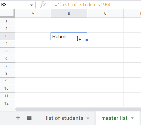
In my case, let’s reference a B4 cell from the sheet named list of students.
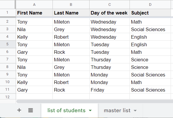
The ready-to-use formula to reference another sheet in Google Sheets will look like this:
='list of students'!B4
Note: if you want to link a range of cells from one sheet to another, just place your cursor on the cell in your data destination worksheet that already contains one of the above-mentioned formulas (='Sheet_1'!A1 or =Sheet1!A1). Then drag it in the direction of your desired range. For example, if you drag it down , the data from these cells will automatically be displayed in your spreadsheet. The same can be done in any other possible direction of your current document.
How to link cell from the current sheet to another tab in Google Sheets
Follow this guide to reference data from the current and other sheets:
- Open a sheet in Google Sheets.
- Place your cursor in the cell where you want the referenced data to show up.
- Use one of the formulas below :
To link a range of cells from the current sheet, use the following formula:
={cell-range}
Where cell-range is the range of cells from your current active sheet. Use curly brackets for this argument.
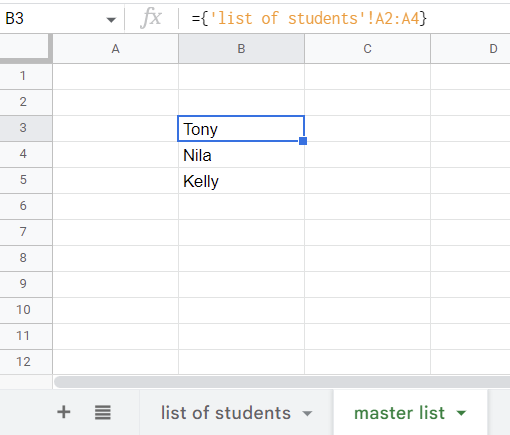
Use the following formula to link to another tab in Google Sheets:
={Sheet1!cell-range}
Where Sheet1 is the name of your referenced sheet and cell-range is a specified range of cells that you want to import data from. Use curly brackets for this argument.
Note: don’t forget to put the sheet’s name in single quotes if it includes spaces or other characters like ):;”|-_*&, etc.
Here is what it looks like in my example:
#6 – How to link columns in Google Sheets
Basically, to link columns in Google Sheets, you need simply to select a range of cells that constitute a column or a few columns and reference them as we described above. However, there is a slightly better way to do this.
How to link a column from one sheet to another tab in Google Sheets
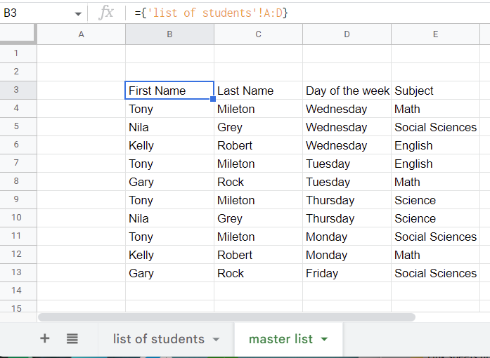
To link a column or columns from one sheet to another tab in Google Sheets, use the following formula:
={Sheet1!columns}
Where Sheet1 is the name of your referenced sheet and columns is a range that specifies that you will pull the data from the A column. Use curly brackets for this argument.
In my case, the ready-to-use formula to reference another sheet in Google Sheets will look like this
={'list of students'!A:D}
#7 – How to link rows in Google Sheets
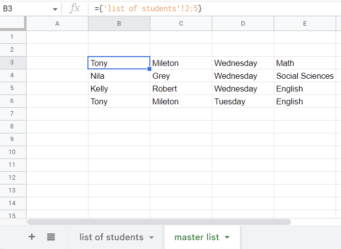
To link a row or rows from one sheet to another tab in Google Sheets, use the following formula:
={Sheet1!rows}
where Sheet1 – is the name of your referenced sheet and rows is a range which specifies the rows which you refer to. Use curly brackets for this argument.
In my case, the ready-to-use formula to reference another sheet in Google Sheets will look like this
={'list of students'!2:5}
Which option works best in Google Sheets to link to another sheet or tab?
Below I have put together a comparison table that briefly explains the pros and cons of the use of the native functionality vs Coupler.io when connecting data between spreadsheets.
| Native Google Sheets functionality | Coupler.io | |
| Type of Google Sheets data linking | References data | Imports data |
| Big data volumes | May show errors or keep loading data for a long time for big volumes of data. | No issues with importing big volumes of data. |
| Frequency of updates | Almost in real-time | Supports manual (any time) and automatic data refresh on a custom schedule. |
| Time to process calculations | It takes some time to process calculations which may slow down the general performance of a spreadsheet. | No calculations are performed on the spreadsheet side. Coupler.io pulls the static data over to your worksheet. |
| Performance in spreadsheets heavily loaded by formulas | Decent. If the total number of formulas in a spreadsheet (including IMPORTRANGE) draws nearer to fifty, the loading speed and the general performance of the document will deteriorate. | Great! It makes no difference for Coupler.io how many formulas you have in your spreadsheet. It will not slow down your worksheet. |
| Managing permissions / access to import data | Granting permissions is performed per every IMPORTRANGE formula separately, which makes it difficult to manage them in bulk. | Managing account connections is available under Coupler.io GSheets importer settings. So, you just create one connection and use it across the entire document. |
| Automatic data backup | IMPORTRANGE syncs the data source and data destination sheets, showing the live data in the latter. So, once the information in the source disappears, it gets automatically removed from your destination sheet as well. | Coupler.io can automatically back up your data and keep it safe in a destination sheet. |
If you’re interested in the comparison of IMPORTRANGE vs. Coupler.io in terms of linking spreadsheets, check out our dedicated blog post on IMPORTRANGE Google Sheets.
Google Sheets to Google Sheets is not the only integration provided by Coupler.io.
Automate data export with Coupler.io
Get started for freeCan I import data in Google Sheets from another sheet including formatting?
Unfortunately, neither of the options above will let you import the formatting of the cell(s) when you reference another Google Sheets workbook. The logic of IMPORTRANGE, FILTER, and other Google Sheets native options does not entail the actual transfer of data. They only reference and display data from the source cells. Coupler.io is the only option that copies the data from the source, but it only imports the raw data without any formatting. At the same time, you can use Coupler.io to link Excel files, as well as Excel and Google Sheets.
BUT you can always use the benefits of Google Apps Script to create a custom function for your needs. For example, the following script will let you transfer data from one sheet or spreadsheet to another:
function importTable() {

  // Source spreadsheet
  var srcSpreadSheet = SpreadsheetApp.openById("insert-id-of-the-source-spreadsheet");
  var scrSheet = srcSpreadSheet.setActiveSheet(srcSpreadSheet.getSheetByName("insert-the-source-sheet-name"));

  // Destination spreadsheet
  var destSpreadSheet = SpreadsheetApp.openById("insert-id-of-the-destination-spreadsheet");
  var destSheet = destSpreadSheet.setActiveSheet(destSpreadSheet.getSheetByName("insert-the-destination-sheet-name"));
  destSheet.clear();

  // Get data and formatting from the source sheet
  var range = scrSheet.getRange(1, 1, 48, 32);

  var values = range.getValues();
  var background = range.getBackgrounds();
  var banding = range.getBandings();
  var mergedRanges = range.getMergedRanges();
  var fontColor = range.getFontColors();
  var fontFamily = range.getFontFamilies();
  var fontLine = range.getFontLines();
  var fontSize = range.getFontSizes();
  var fontStyle = range.getFontStyles();
  var fontWeight = range.getFontWeights();
  var horAlign = range.getHorizontalAlignments();
  var textStyle = range.getTextStyles();
  var vertAlign = range.getVerticalAlignments();

  // Put data and formatting in the destination sheet
  var destRange = destSheet.getRange(1, 1, 48, 32);

  destRange.setValues(values);
  destRange.setBackgrounds(background);
  destRange.setFontColors(fontColor);
  destRange.setFontFamilies(fontFamily);
  destRange.setFontLines(fontLine);
  destRange.setFontSizes(fontSize);
  destRange.setFontStyles(fontStyle);
  destRange.setFontWeights(fontWeight);
  destRange.setHorizontalAlignments(horAlign);
  destRange.setTextStyles(textStyle);
  destRange.setVerticalAlignments(vertAlign);

    // Iterate through to put merged ranges in place
  for (var i = 0; i < mergedRanges.length; i++) {
    destSheet.getRange(mergedRanges[i].getA1Notation()).merge();
  }

  // Iterate through to get the column width of the source destination
  for (var i = 1; i < 18; i++) {
    var width = scrSheet.getColumnWidth(i);
    destSheet.setColumnWidth(i, width);
  }

  // Iterate through to get the row heighth of the source destination
  for (var i = 1; i < 27; i++){
    var height = scrSheet.getRowHeight(i);
    destSheet.setRowHeight(i, height);
  }

}
You need to go Extensions > Apps Script. Then insert the script in the Code.gs file and specify the required parameters:
- ID of the source and destination spreadsheets
- Names of the source and destination sheets
(If you’re importing data between sheets, the source and destination spreadsheet ID will be the same)
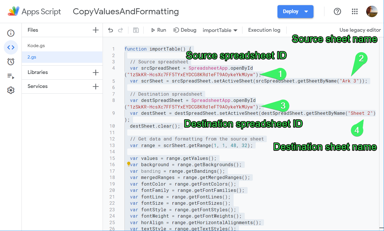
When ready, click Run and your data including formatting will be imported into the destination sheet.
Note: This solution may not be a fit for your project, so you’ll need to update the script whatever you require.
What to choose to reference data from other sheets or tabs
There is no one-size-fits-all solution and you have to be careful when going one way or another. Whether you are looking to link sheets, spreadsheets, create combined views, or back up documents – be sure to consider all the advantages and disadvantages of both and pick the right option for you to achieve the best result.
If you only have a few records in your spreadsheet and little formulas, then you might go for a formula-based approach including IMPORTRANGE provided by Google Sheets. This will work for regular reporting or low-level analytics.
However, if you possess lots of data and there are multiple calculations in your document, then you should opt for the import data method instead of referencing it. Coupler.io will be a more stable solution in this case. It will provide failsafe data transfer and ensure that you have access to the data even if the data source is damaged or not available. Choose wisely and good luck!