Let’s say you opened your Google spreadsheet and discovered that all your IMPORTRANGE formulas were not working. The previously imported data disappeared and refreshing won’t help get it back. Many users have already suffered from this drawback known as IMPORTRANGE Google Sheets not working. To avoid it, you’d better use an alternative solution, which turns your spreadsheet into a sort of relational database. We’ll show you how to do this a bit later. But for now, let’s troubleshoot your IMPORTRANGE formula and fix the current error.
Most common IMPORTRANGE internal errors
The common Google Sheets IMPORTRANGE errors are #ERROR! and #REF!. You can either read how to fix them or watch the video tutorial on the IMPORTRANGE function or do both. It’s up to you 🙂
#1 IMPORTRANGE #ERROR! – Formula parse error IMPORTRANGE
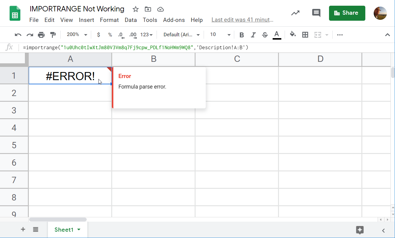
It’s kid’s stuff! Formula parse error means that you’ve made a mistake in the IMPORTRANGE formula syntax.
How to fix
Verify the formula syntax. Make sure also to validate the spreadsheet URL or ID, quotation marks, as well as the range string. These are the most common reasons for the formula parse error.
#2 IMPORTRANGE #REF! – Permission error or You don’t have permissions to access that sheet
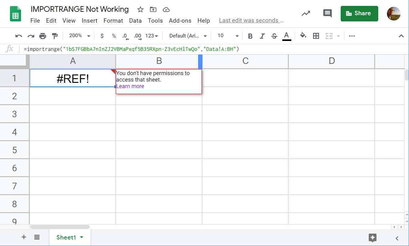
This error states that “You don't have permissions to access that sheet.” In most cases, this means that you’re trying to import a dataset from an unshared Google Sheets doc that is not stored on your Google Drive.
How to fix
Share the source spreadsheet with the owner of the target spreadsheet or make the file shareable with “Anyone with the link.“
Formula parse errors and permission errors are the most common IMPORTRANGE failures. We’ll cover other mishaps later but first, let’s find out how you can avoid and prevent IMPORTRANGE from any failure.
How to fix all IMPORTRANGE errors at once and never face them again
The main issue with IMPORTRANGE errors is that you don’t have access to your data. The reason is that IMPORTRANGE does not actually import data but refers to it. So, when the formula is broken, your data from another spreadsheet becomes unavailable.
So, the best way to solve the IMPORTRANGE Google Sheets not working issue is to have your data imported. IMPORTRANGE can’t do this but the Google Sheets integration by Coupler.io can. It connects the source and destination spreadsheets and automated data flow between them.
With this integration, you can import data from an entire sheet or a specified data range. You can also combine data from multiple sheets or spreadsheets (different Google Sheets files) into one.
The Google Sheets integration is available as a web app and a Google Sheets add-on. For the latter, you’ll need to install the Coupler.io add-on from the Google Workspace Marketplace.
How to import data using Google Sheets integration to avoid IMPORTRANGE issues?
Click Proceed in the form below – this will create a Google Sheets importer to import data between spreadsheets.
You’ll be prompted to sign up with your Google account for free. After that, complete 4 simple steps:
- Step 1. Extract data: Specify the source spreadsheet from which to extract data.
- Step 2. Transform data: Preview and transform the data to load to the destination spreadsheet.
- Step 3. Load data: Specify the destination spreadsheet where to import data.
- Step 4. Schedule importer: Set up a schedule for automatic data refresh to have up-to-date information.
Here is what the configured Google Sheets integration may look like:
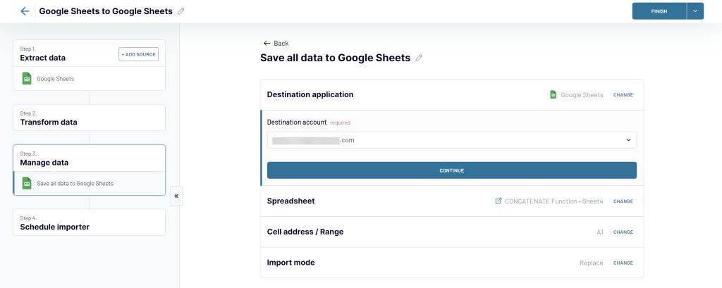
Once you run your importer, it will import data from the source spreadsheet to the destination one and will refresh the data according to the specified schedule.
Coupler.io is not limited to Google Sheets integration. It supports 50+ other applications from which you can load data to the preferred destination be it spreadsheets, BI tools, or data warehouses.
Other IMPORTRANGE hiccups that you may encounter
#3 IMPORTRANGE #REF! – Allow access or You need to connect these sheets
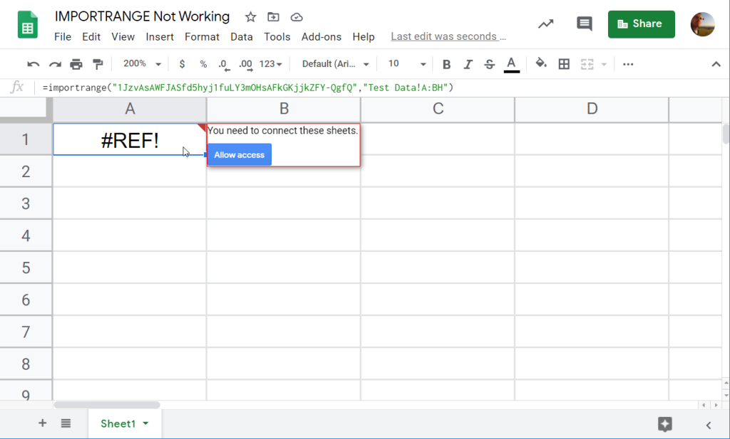
This is more of a warning than an error. When you import a range from an unshared spreadsheet stored on your Google Docs for the first time, IMPORTRANGE will require you to connect the source and the target sheets.
How to fix
Click the Allow access button to connect the sheets.
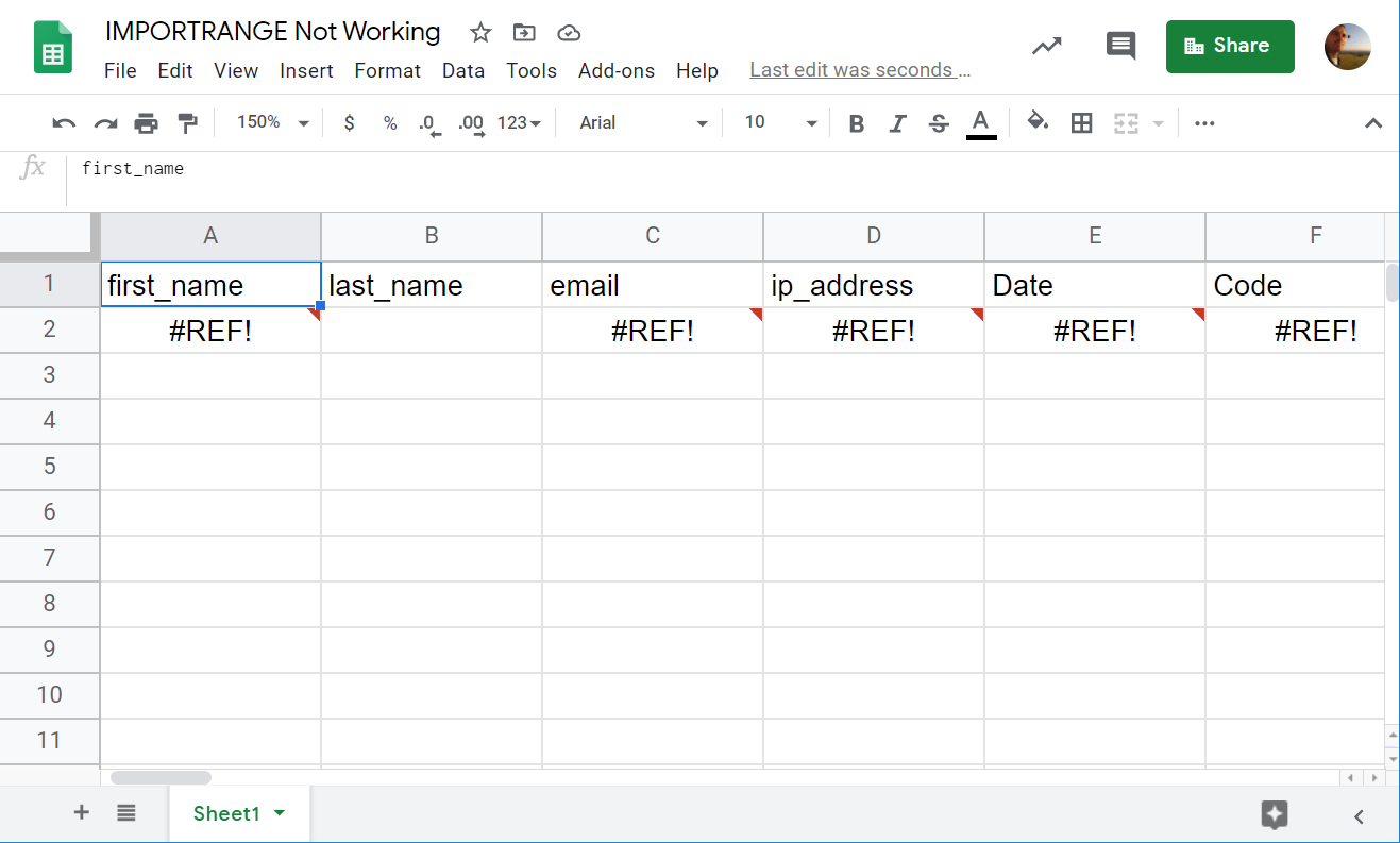
#4 IMPORTRANGE #Error! – IMPORTRANGE Result too large

You’ll see this error when you’re importing too many cells. Unfortunately, the exact amount of cells you can import with IMPORTRANGE is undisclosed. In our example, we tried to import 60 columns and 6000 rows (360,000 cells). After we decreased the data range to 4300 rows (258,000 cells), the IMPORTRANGE formula worked.
How to fix
Split the data range into two or more pieces, either vertically (by rows) or horizontally (by columns). Nest IMPORTRANGE formulas for each piece within the ARRAYFORMULA function as follows:
For horizontally split pieces (use commas between IMPORTRANGE formulas):
=ARRAYFORMULA({IMPORTRANGE("sheet-id","data-range-piece#1"),IMPORTRANGE("sheet-id","data-range-piece#2"),...})For vertically split pieces (use semicolons between IMPORTRANGE formulas):
=ARRAYFORMULA({IMPORTRANGE("sheet-id","data-range-piece#1);"IMPORTRANGE("sheet-id","data-range-piece#2");...})For example, here is a failed IMPORTRANGE formula:
=importrange("1bS7FGBbA7nInZJ2VBMaPxqf5B35RXpn-Z3vEcHlTwQo","Data!A:BH")
We split the range of cells "Data!A:BH" by columns into "Data!A:AM" and "Data!AN:BH" and applied the following formula:
=arrayformula({importrange("1bS7FGBbA7nInZJ2VBMaPxqf5B35RXpn-Z3vEcHlTwQo", "Data!A:AM"),importrange("1bS7FGBbA7nInZJ2VBMaPxqf5B35RXpn-Z3vEcHlTwQo", "Data!AN:BH")})
#5 IMPORTRANGE #REF! cannot find range or sheet for imported range
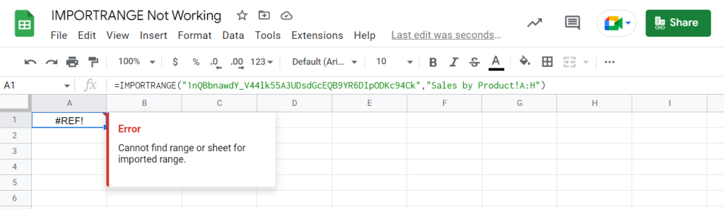
If you see the #REF! Error with a note “Cannot find range or sheet for imported range”, it’s most likely that either the sheet name is misspelled or you entered the wrong range.
If the formula worked before and then you saw this error, then the sheet was probably renamed or deleted, or the spreadsheet was removed.
How to fix
First of all, double-check the name of the sheet (both in the IMPORTRANGE formula and your source spreadsheet) and the range you entered. In the vast majority of cases, this is the reason for this internal IMPORTRANGE error.
#6 IMPORTRANGE #REF! – Frozen formulas
This glitch is well-known among Google Sheets users. Yesterday, your IMPORTRANGE formulas worked well. Today, they return #REF! and seem to be broken for no reason.
It happens randomly and sometimes fixes itself. For many years, Google has failed to find a stable solution to get rid of this ongoing issue with IMPORTRANGE.
How to fix
There are many approaches to fixing this issue:
- Hard refresh of the sheet and/or browser
- Re-adding the IMPORTRANGE formula to the same cell (use the Google Sheets shortcuts Ctrl+X and then Ctrl+V or clear the cell and use Ctrl+Z to restore it)
- Nest IMPORTRANGE with IFERROR
=IFERROR(IMPORTRANGE("sheet-id","range"))The sheet will reattempt the data import again and again automatically.
- Use the
=now()trick:- Insert a NOW formula (
=now()) in a random cell of the source and target spreadsheets - Insert an IMPORTRANGE formula that references the NOW formula of the other spreadsheet
- Go to File => Spreadsheet settings => Calculation and select Recalculation “On change and every minute“
- Insert a NOW formula (
- Split large chunks of data into pieces using ARRAYFORMULA + IMPORTRANGE, just like with Error! Result too large.
If you know other solutions/approaches to dealing with IMPORTRANGE #REF!, please share them with us to include in the article.
If you need more information about this function, check out our IMPORTRANGE Tutorial.
How frequently is IMPORTRANGE Google Sheets not working?
Although IMPORTRANGE is an awesome function in Google Sheets to link to another sheet, its reliability is arguable. Google does not publicly disclose information on the failures of individual functions. However, like any software, you can experience occasional errors when using Google Sheets. So, we can’t be sure how frequently IMPORTRANGE Google Sheets is not working.
Meanwhile, if you ask StackOverflow about any errors or failures associated with IMPORTRANGE, you’ll get many results starting from 2015. As a rule, such bugs or glitches are solved within a day or two. It’s not a long term but it’s much better not to experience this at all.
Forget about IMPORTRANGE failures with Coupler.io
Let’s say you have 100 source sheets from which you import data to 30 sheets using IMPORTRANGE formulas. From the target sheets, you import data to another 10 sheets again with IMPORTRANGE. If all these formulas are stuck, you will face issues with troubleshooting and fixing them!
IMPORTRANGE is a function, and it takes some time to process calculations, which slows down the general performance of a workbook. Instead, you can use the IMPORTRANGE alternative – Google Sheets integration. It is free of the mentioned IMPORTRANGE performance issues since no calculations are performed in the spreadsheet. It pulls the static data and saves it in your spreadsheet, just in case anything goes wrong.
This is why we recommend you consider Coupler.io as an IMPORTRANGE Google Sheets alternative for your project. Check it out and good luck with your data!