Tracking expenses is the only way to make sure that your money does not go down the drain. The idea is pretty simple: you need to categorize expenses by category and analyze how much you spend on each. Examples of categories include food, insurance, utilities, etc. Based on the analysis, you’ll be able to decrease expenses and increase savings. Does it sound enticing? Then check out the personal Google Sheets expense tracker template, which is available for your use for free.
Google Sheets spending tracker template explained
The expense tracker was designed in Google Sheets and consists of two sheets:
- Expense Tracker – the sheet with the tracker itself: it allows you to filter out expenses by categories according to the selected period. This sheet also contains the breakdown of income and expenses by categories/months.
- Import your income/expenses – the sheet where you can manually or automatically import data about your revenues and expenses.
Expense Tracker
On the Expense Tracker sheet, you’ll see the grouped rows for income and expenses. Click on “+” to expand each of them.
Here you need to specify your categories for income and expenses. If the default ones are okay, then skip this step.
The expense tracker Google Sheets looks as follows:
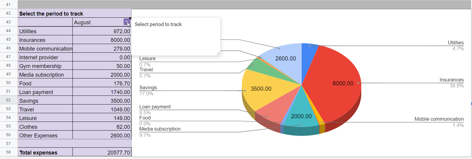
It lets you filter out expenses by a certain period. Click on the B43 cell and choose the period from the drop-down list. The pie chart will update once you change the period to filter by.
Import your income/expenses
The personal Google Sheets expense tracker template will work after you feed data into it. For this, you need to go to the Import your income/expenses sheet. It has 5 columns:
- Date – specify the date of your income/expense. Click on the cell and select the date.
- Period – a technical field that extracts the name of the month from the date you specify in the Date column.
- Income – select the type of income from the drop-down list. (The list consists of the income categories from the Expense Tracker sheet)
- Expense – select the type of expense from the drop-down list. (The list consists of the expense categories from the Expense Tracker sheet)
- Amount – specify the amount of income/expense in the currency you need.
You can input the expense/income data manually. It’s convenient for the expenses in cash. For non-cash spending and revenues, it’s better to import transactions from your bank. This can be done automatically with Coupler.io. The only prerequisite for this is checking the API available at your bank.
How to import bank transactions to the Google Sheets expense tracker template
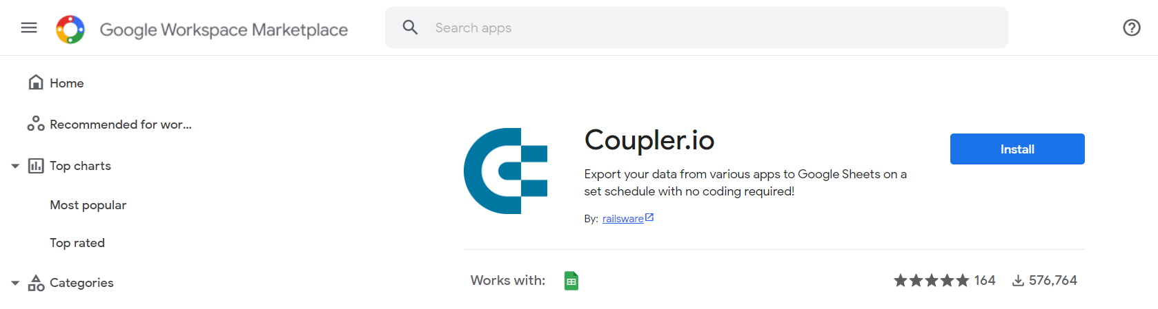
We will fetch data from a banking web API using Coupler.io. It is a tool that allows users to automatically import data from multiple sources, such as Pipedrive, Xero, and others to Google Sheets, Excel, and BigQuery. You can use the Coupler.io web app or install the Google Sheets add-on from the Google Workspace Marketplace. To connect to the web APIs, Coupler.io provides a JSON integration. You can learn more about how it works in this API to Google Sheets guide. Let’s begin.
To start your data integration journey, select the source and destination apps in the form below and click Proceed.
- Connect your data source: Connect your source app or specify the parameters based on the API documentation of your bank.
- Organize your data: Prepare your data and specify where to load it .
- Configure importer’s schedule settings: Set up the Automatic data refresh on a schedule.
As an example, check out the parameters I used to set up the integration with Monobank to export bank transactions to spreadsheets:
| Parameter | Value |
|---|---|
| Title | monobank transactions |
| JSON URL | https://api.monobank.ua/personal/statement/{account}/{from}/{to} |
| HTTP Method | GET |
| HTTP Headers | X-token:{api-token} |
| Sheet name | monobank transactions |
| Automatic data refresh frequency | daily |
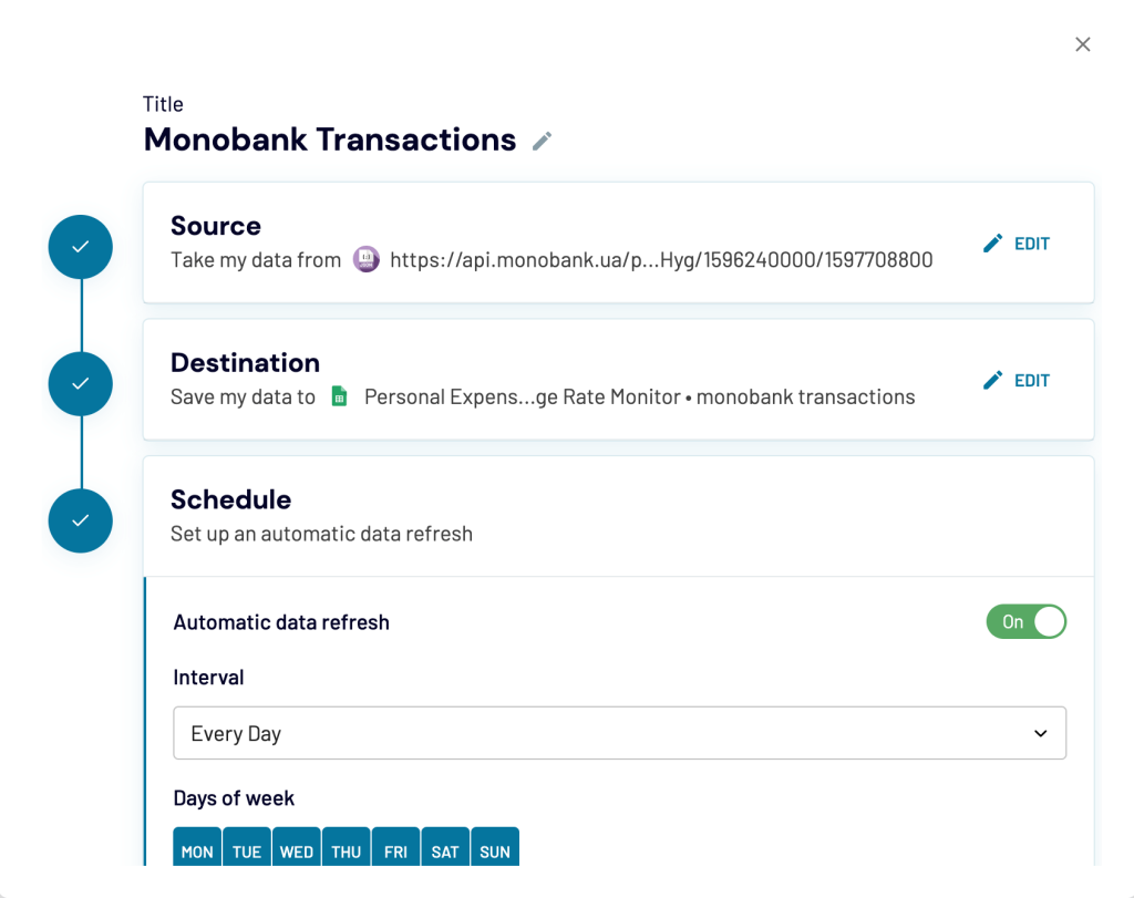
Once the parameters are set up, click Save & Run to make the initial data import. After that, Coupler.io will refresh the data automatically every day.
Query the spending data to your daily expense tracker in Google Sheets
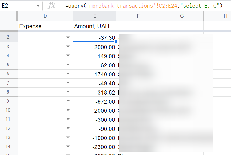
With the raw data imported to Google Sheets, you need to query it to the Import your income/expenses sheet of your daily expense tracker Google Sheets. In our case, these are three columns: time, description, and amount.
We applied the following QUERY formula in the E2 cell to reference the amount and description columns:
=query('monobank transactions'!C2:E24,"select E, C")
Learn more about the power of the QUERY Function Google Sheets.
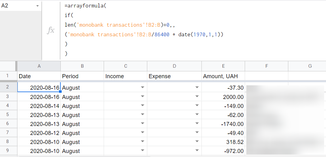
The values in the time column are in the unix epoch time format (in seconds). To convert them into real data, apply the following formula based on the ARRAYFORMULA + DATE functions in the A2 cell:
=arrayformula(
   if(
      len('monobank transactions'!B2:B)=0,,
      ('monobank transactions'!B2:B/86400 + date(1970,1,1))
   )
)
86400– the number of seconds in a day (24 hours x 60 minutes x 60 seconds)date(1970,1,1)– the date value for the Unix Epoch, January 1, 1970 (25569)
The only thing left is to allocate categories (Income or Expense) to the imported data. In our case, we must do this manually. Once you map the expenses/income data, it will appear in the Expense Tracker sheet of the expense tracker Google Sheets.
This is possible due to the following formula that links cells between sheets:
=iferror(
   sum(
      filter(
         'Import your income/expenses'!$E$2:$E,
         'Import your income/expenses'!B2:B = {cell with the name of the month},
         'Import your income/expenses'!C2:C = {cell with the type of income/expense}
      )
   )
)
Now, let’s get back to the tracker.
Monitor your spending with the expense tracker in Google Sheets
Go to the tracker and select the period to track. For example, we selected August, and all the imported expenses in August have been returned:
The pie chart will update accordingly. The tracker has two fundamental elements:
- Period selector with the drop-down list. To make this, you need to apply data validation (list from a range).
- Filter formula which extracts the data based on the criteria specified in the period selector. Here is how it looks:
=filter(A19:N39,A1:N1=B43)
Read our tutorial to learn more about the FILTER Function in Google Sheets.
Note: the pie chart works with absolute values only. In our case, the imported bank transactions were both negative (expenses) and positive (income). After the mapping, it’s recommended to use the ABS function to get absolute values for minus numbers (or ARRAYFORMULA + ABS for an entire column).
Daily or monthly expense tracker in Google Sheets is better?
Frankly speaking, I was not used to tracking my spending in detail. As many of us do, I relied on my memory. My expenses monitoring resembled “$200 for sneakers are too much..maybe in a couple (not Coupler:) of months.“

Automate financial reporting with Coupler.io
Get started for freeNow that my spending data is structured, I know exactly what kind of expenses I can afford and how this can affect my cash balance. As for the tracking frequency that works better, it seems that it depends on the tracking goal. The tracker introduced in the article is a monthly expense tracker Google Sheets. However, you can start with daily tracking to optimize your expenses at a low level. Then after a few months, you can switch to monthly tracking.
I hope that my experience and this expense tracker template will help you as well. Good luck with your data!