Working with numbers, invoices, reporting documents, prices, and sales requires a lot of attention and accuracy. Therefore, SUMIF in Excel helps perform multiple tasks quickly and efficiently. Let’s take a closer look at syntax, usage, and formulas based on some examples.
One criterion Excel SUMIF example, values, and usage
Sometimes, a person wants to do some counting work by applying the SUMIF Excel function. It operates with one criterion and has a set syntax.
=SUMIF (range, criterion, [sum_range])range– these are all of the cells being evaluated: from the first with a particular condition to the last.criterion– it is a condition which may include names of people, products, goods, dates, months, etc.sum_range– it is the collection of values that will be summarized.
For example, look at the spreadsheet:
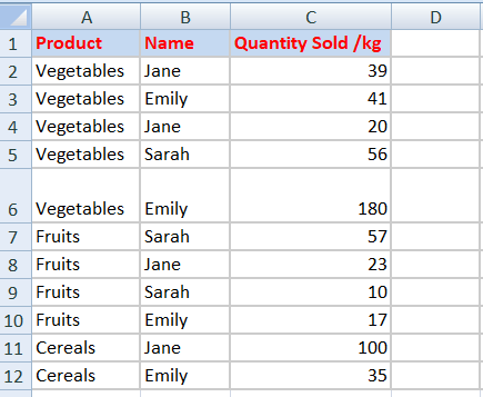
Using the SUMIF formula, you can determine the indicators that you ought to evaluate with only one criterion:
- Total quantity of products that people buy
- Total quantity of products that Jane (or Emily, or Sarah) bought
- The amount of each product group
Sometimes, it is necessary to import data from applications and sources into Excel, Google Sheets, or BigQuery. We can do this task by using the Coupler.io tool if the data is in many outer sources, such as Shopify or Jira. Thus, you get the necessary data collected all together in tables.

For example, you usually store data on Pipedrive, but using SUMIF in Excel with multiple criteria is necessary. So, you can export the data to a workbook saved in OneDrive.
You do not need any programming skills for setting up an integration with Excel. The whole process is easy and requires only a few steps. In addition, you can configure updates automatically, so your data can update according to your schedule if necessary.
SUMIF Function in Excel with multiple criteria and with one criterion – The difference
You can’t use the SUMIF function for multiple criteria. For this purpose, you’ll need SUMIFS.
The SUMIF function differs in formula usage, syntax, and purpose from the SUMIFS function. The latter has a slightly more complex syntax
=SUMIFS (sum_range, criterion_range1, criterion1, [criterion_range2, criterion2],…).Sometimes Excel users confuse the two functions. Let’s get a better understanding and compare them. The SUMIF function summarizes only one criterion while SUMIFS performs the calculation with several conditions.
However, many people claim to use the Excel SUMIF function with multiple criteria. This statement is not entirely true. What the majority of these people are actually using for their calculations is the SUMIFS function. Take another look at the distinctive characteristics below:
| SUMIF | SUMIFS |
|---|---|
| Sums up by one criterion | Sums up by multiple positions |
Starts with range | Starts with sum_range |
| Sum range may not always coincide with the cells number | The number of rows and columns must always be the same as the sum range |
| Fewer characters and operators | More characters and operators |
Applying Excel SUMIF multiple criteria cell reference
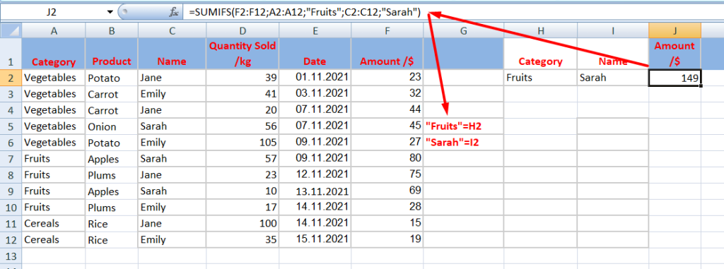
The formulas may contain words, meanings, names, etc. However, Excel SUMIF with multiple criteria doesn’t always require such extensive use of words. There is another solution that can be used instead of words, it is cell reference for the criterion parameter. Here is an example with words:
=SUMIFS(F2:F12,A2:A12,"Fruits",C2:C12,"Sarah")
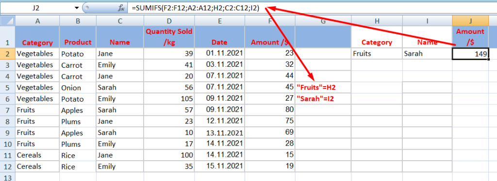
So, let’s replace the formula with cell links instead. The outcome will remain the same:
=SUMIFS(F2:F12,A2:A12,H2,C2:C12,I2)
How to use SUMIF in Excel with multiple criteria – widespread examples
We have already considered the theory of function use, its differences, and syntax. Now, let’s start the practical work of the SUMIF function in Excel with multiple criteria. Although there is no single, fixed formula into which we put our data, we will look at examples of the function in various cases, taking into account several conditions, logic, one or more columns, dates, and so on.
SUMIFS multiple criteria column and row
A person working within finance, accounting, or management niches constantly faces new accounts and certain conditions. Sometimes, summation requires consideration of multiple conditions. What parameters does the syntax include?
- Consider the first three mandatory parameters:
sum_range,criterion_range, andcriterion. - You can add more criteria after these three arguments if needed (e.g., words, numbers, cell links, etc.).
- Remember to use wildcards and operators, such as
>,<,<>,=*,?,>=, and<=.
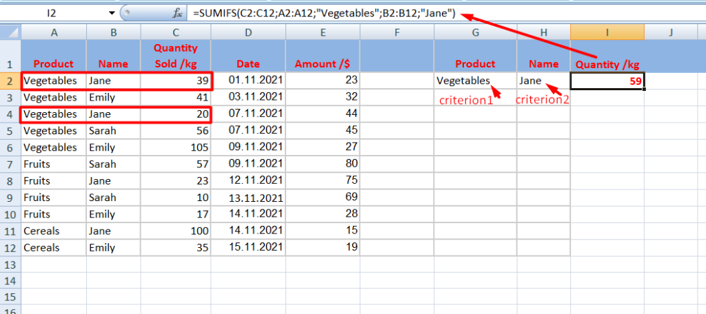
Look at the table where we calculate not only the total of some goods but also the quantity of vegetables Jane purchased. So, "vegetables" is our 1st criterion and "Jane" is the 2nd.
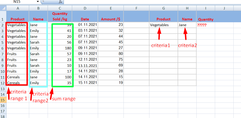
What formula will we get as a result? Using the following example, we need to know the quantity of vegetables Jane bought.
=SUMIFS(C2:C12,A2:A12,"Vegetables",B2:B12,"Jane")
AND logic: Excel conditional SUMIF with multiple criteria
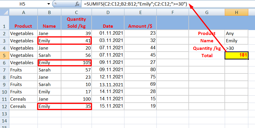
You can sum up many more conditions and criteria if you use the SUMIFS function that is based on AND logic. Look at another sample with comparison operators. Let’s find out how many products Emily has bought that weigh more than 30 kilograms.
=SUMIFS(C2:C12,B2:B12,"Emily",C2:C12,">=30")
OR logic: Excel formula for SUMIF with multiple criteria
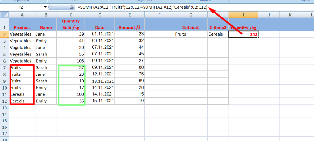
We can add SUMIF functions by dividing each criterion separately or multiple criteria together using an array constant. The whole process is based on OR logic. Take, for instance, the summation separately for each criterion. Imagine that you need to find the total amount of fruit and cereals people have bought.
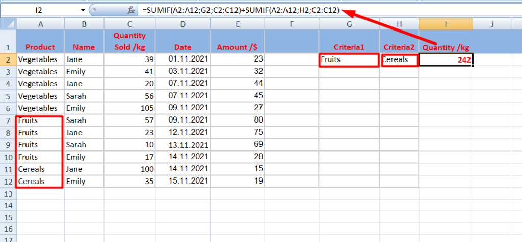
=SUMIF(A2:A12,"Fruits",C2:C12)+SUMIF(A2:A12,"Cereals",C2:C12)
You can write G2 and H2 instead of textual names. This combination is also correct and doesn’t change the result.
What are SUMIFS multiple criteria for different columns?
People often use large tables containing a lot of data. Sometimes they need to count by different categories so SUMIFS can simplify this task by allowing you to summarize the results of several columns. Let’s analyze the function based on our situation.
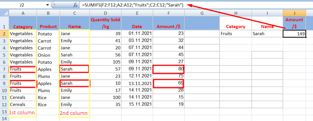
We have a table with categories, products, people, quantity sold, dates, and amount. We can calculate the total quantity of potatoes, carrots, or other categories of goods one of the buyers purchased. Additionally, you can calculate the cost of products purchased by one or more buyers. Let’s sum up the price of the fruits that Sarah bought.
=SUMIFS(F2:F12,A2:A12,"Fruits",C2:C12,"Sarah")
How do you use Excel SUMIFS with multiple criteria in the same column?
Excel users can look at another example of counting values in one column. We can use SUMIF + SUMIF (already written above) or SUM nested with SUMIFS. Consider the last example – it would be more convenient if we used many criteria in the formula.
Let’s imagine that we need to define the total cost of plums and apples. Looking at the screenshot, you can see that these two products are in the same column. We will calculate their total price using Excel SUMIF with multiple criteria.
=SUM(SUMIFS(F2:F12,B2:B12,{"Apples";"Plums"}))
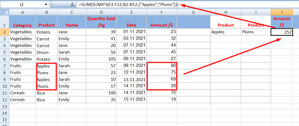
Thus, we summed up the products in one column, using Excel SUMIF with multiple criteria.
How to use an Excel SUMIF with multiple criteria in an array formula?
Adding SUMIF functions is a simple solution when summing up individual criteria. However, such a process is too complex and inconvenient if there are many OR conditions. It also takes a long time to write out the formula. So, a useful alternative would be to use an array argument instead.
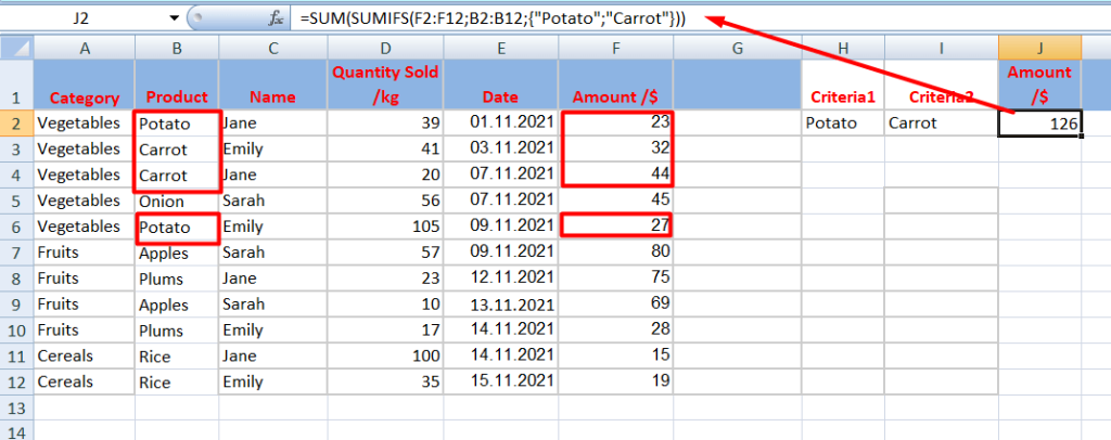
You need to use braces {}, within which you place all of the necessary products (carrot and potato or apples and plums), categories (fruits or vegetables), or other criteria you want to summarize. Also, you can’t write the formula with a cell reference because only the name will fit here. The best choice for this example would be to use SUMIFS and SUM. So, let’s take the example from the table and include some vegetables.
Assume we need to count up the price of either "Carrot" and "Potato" in an array constant. The formula looks like this:
=SUM(SUMIFS(F2:F12,B2:B12,{"Potato";"Carrot"}))
Excel SUMIF multiple criteria date range
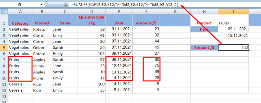
The SUMIF function in Excel with multiple criteria and SUMIFS can perform price calculations taking into account dates. For example, you can determine the value of some products purchased only on certain dates. You can also consider specific periods of time: from one date to another, for only one week or month, etc.
Now, let’s calculate the total cost of fruits purchased in the last five days. Here is the formula:
=SUMIFS(F2:F12,E2:E12,">="&I2,E2:E12,"<="&I3,A2:A12,I1)
How do you summarize with Excel SUMIF multiple criteria horizontal and vertical?
Unfortunately, the SUMIFS function will not help you if you want to summarize values in rows and columns together. You should use SUMPRODUCT for this type of calculation. However, SUMIFS easily summarizes the values horizontally and vertically individually depending on the range you specified.
Value of SUMIFS with multiple criteria
SUMIF and SUMIFS functions are useful for people in many professions because they simplify the calculation process in various situations. However, we do not always have all of the data that we need in one place.
We store various data across multiple applications and resources which are not easy to import into Excel without a special tool like Coupler.io. So, you can start by using the Excel integrations to import your data into a workbook before using our guide to enter the values and data into the formulas.