When you need to sum values with a certain condition, how do you handle it when the criteria are in different tables? Combining Excel’s SUMIF and VLOOKUP functions is one option. In this article, we’ll show you how to do that, including other examples of using both functions together in one formula!

Automate data import to Excel with Coupler.io
Get started for freeHow to do SUMIF and VLOOKUP together in Excel
You can use VLOOKUP and SUMIF (or SUMIFS for multiple criteria) together in Excel for various purposes—for example:
- VLOOKUP within SUMIF, when you need to sum values based on conditions, but you also have to lookup from another table to get the correct criteria value.
- SUMIF within VLOOKUP, when you need to search for a value based on the total you’ve summed. Another case is when you need to do a lookup by criteria but want a non-numeric value instead of numbers as a result.
- SUMIF + VLOOKUP + another function, for more complex scenarios. For example, you can use SUMIF + VLOOKUP + SUMPRODUCT when you want to sum across multiple sheets then find the approximate match from a lookup table based on the totals you’ve got.
SUMIF and VLOOKUP are both very useful formulas. You can use them in a variety of scenarios (including those not mentioned above). Understanding how each of these functions works is crucial to being able to use them properly when you need them!
If you haven’t used either SUMIF or VLOOKUP, please check out our articles covering the basics of these functions: Excel SUMIF function and Excel VLOOKUP function.
Excel SUMIF + VLOOKUP examples
Now, let’s explore some examples below on how to use Excel SUMIF & VLOOKUP together.
#1: Excel SUMIF with VLOOKUP for looking up the criteria value
Suppose you have the following spreadsheet that contains Orders and Products data in two separate tables. Then, you want to add up the amount for Firecracker and put the result in I3.
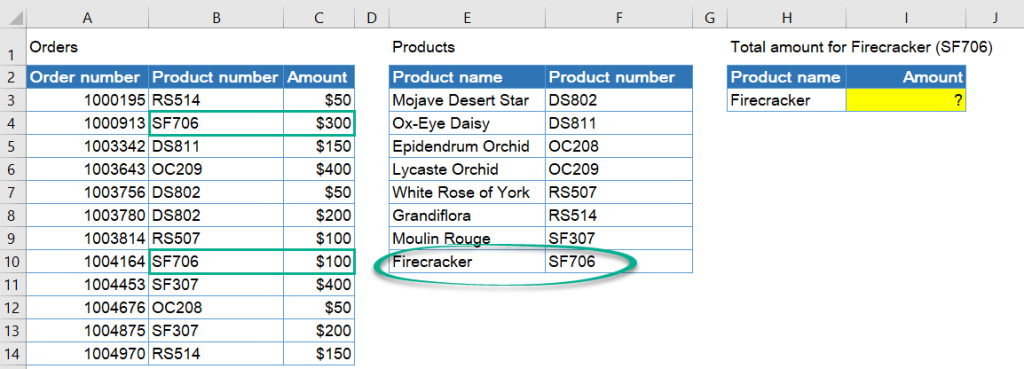
But, as you can see, the Orders table does not have a column for product names. This means that you can’t just sum up the amount for your orders where the product name is equal to Firecracker directly with the SUMIF function.
The solution? You need to get the product number of Firecracker first, then use it as the criteria in your SUMIF function. Here are the steps:
Step 1: Write the VLOOKUP formula in I3 to get the product number of Firecracker.
=VLOOKUP(H3,E3:F10,2,FALSE)
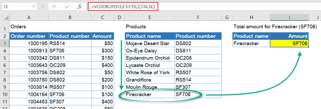
The formula looks for a value that exactly matches “Firecracker” in the first column of the range E3:F10. Then, it returns “SF706” from the second column of the range (column F).
Step 2: Use the VLOOKUP in a SUMIF, as shown below:
=SUMIF(B3:B14, VLOOKUP(H3,E3:F10,2,FALSE), C3:C14)
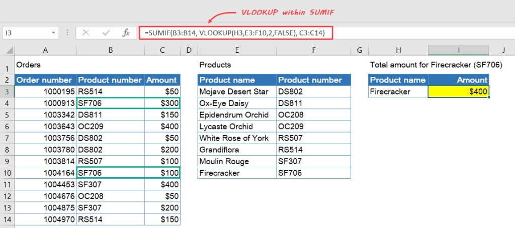
The SUMIF formula adds the amount in C3:C14 where any value in B3:B14 equals “SF706“. You can see the final result in I3, which is $400.
#2: Excel VLOOKUP with SUMIFS to lookup with multiple criteria
For this example, we use a small subset of an Employee dataset stored in Airtable. We exported data from Airtable to Excel using Coupler.io, an reporting and data integration solution. It offers over 70 Microsoft Excel integrations with other apps, such as Airtable, Jira, Shopify, Slack, and many more. Try it out yourself for free. Just select the needed tool in the form below and click Proceed to get started.
Now, with the following Employee data, suppose you want to find an employee’s email address based on their first name, last name, and department.
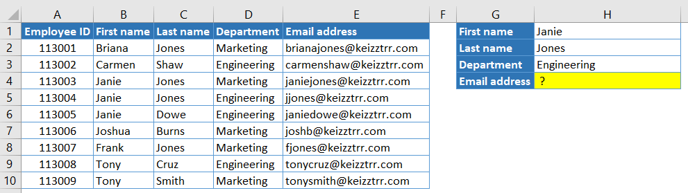
Assume that each Employee ID value is unique, and each department does not contain any employees with the same full name.
It would be easy if you only need to lookup based on the Employee ID. You could just use VLOOKUP, and it’s done. But unfortunately, you can’t use VLOOKUP because you need to do a lookup on multiple columns.
So, what’s the solution? Well, luckily, you can combine both Excel VLOOKUP and SUMIFS to get the result you want! Use SUMIFS to get the ID of the specified employee based on their first name, last name, and department. Then, use that ID in a VLOOKUP function to return the email address.
Here are the steps:
Step 1: Use SUMIFS to get the ID of the specified employee:
=SUMIFS(A2:A10,B2:B10,H1,C2:C10,H2,D2:D10,H3)
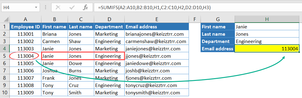
As you can see, the above formula in H4 returns the ID of Janie Jones from the Engineering department, which is 113004.
Step 2: Use the SUMIFS within a VLOOKUP to find an email address based on the employee ID, as shown below:
=VLOOKUP(SUMIFS(A2:A10,B2:B10,H1,C2:C10,H2,D2:D10,H3),A2:E10,5,FALSE)
The VLOOKUP formula above uses the result of the SUMIFS function as the lookup value. It then finds the exact match in range A2:E10 and returns “jjones@keizztrr.com“, which is located in the fifth column of the range.
#3: Excel SUMIF + SUMPRODUCT + VLOOKUP to sum values across multiple sheets
Suppose you have the following spreadsheet with four worksheets: Summary, Apr, May, and Jun. In the Summary worksheet, you want to calculate the quarterly bonus for each salesperson using the lookup table on the right.
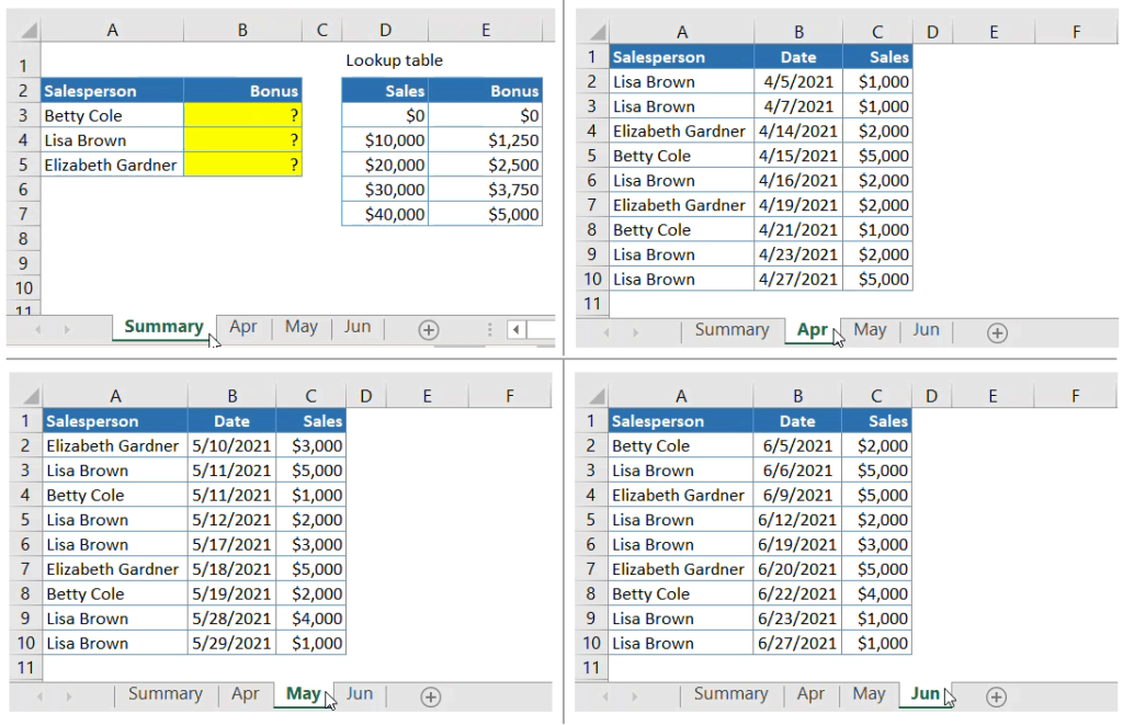
In this scenario, you will sum up the sales across Apr, May, and Jun for each salesperson. With these numbers, you will be able to determine the bonuses based on the idea of breakpoints, as follows:
| Total sales | Bonus |
|---|---|
| $0 – $9,999 | $0 |
| $10,000 – $19,999 | $1,250 |
| $20,000 – $29,999 | $2,500 |
| $30,000 – $39,999 | $3,750 |
| >= $40,000 | $5,000 |
So, let’s say you do the math manually and find that Lisa Brown made $38,000 in total sales, Betty Cole made $15,000, while Elizabeth Gardner was more successful with her total sales of $22,000. So, based on their performance, they will be receiving bonuses of $3,750, $1,250, and $2,500, respectively.
Doing calculations manually is not always fun. So, let’s see the below steps to calculate the bonus using formulas in Excel:
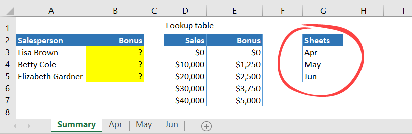
Step 1: In the Summary sheet, list all the sheet names you will sum. For example, in G2:G5, as shown below:
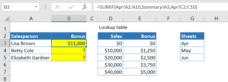
Step 2: For the first salesperson, write a SUMIF Formula for one sheet only – for example, Apr.
=SUMIF(Apr!A2:A10,Summary!A3,Apr!C2:C10)
Step 3: Wrap the SUMIF inside SUMPRODUCT.
=SUMPRODUCT(SUMIF(Apr!A2:A10,Summary!A3,Apr!C2:C10))
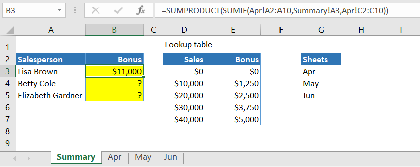
We need to do this because, in the next step (Step 4), we’re going to use SUMIF to sum across multiple sheets using the sheets’ reference in G2:G5. The SUMIF will return an array, so we use SUMPRODUCT to make sure that everything will get summed up correctly.
Step 4: Sum across the sheets by using the list of sheet names as a reference. Let’s use an absolute range — so, in this case,
- Replace
Apr!A2:A10withINDIRECT("'"&$G$3:$G$5&"'!"&"A2:A10") - Replace
Apr!C2:C10withINDIRECT("'"&$G$3:$G$5&"'!"&"C2:C10")
The complete formula will be:
=SUMPRODUCT(SUMIF(INDIRECT("'"&$G$3:$G$5&"'!"&"A2:A10"),Summary!A3,INDIRECT("'"&$G$3:$G$5&"'!"&"C2:C10")))
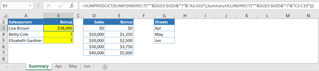
From the result in B2, you can see that Lisa Brown’s total sales for the months of April, May, and June were $38,000 in total. Her bonus will be calculated based on this amount.
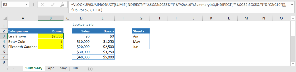
Step 5: Calculate the bonus by finding the approximate matches in the lookup table. To do this, wrap the SUMPRODUCT inside VLOOKUP:
=VLOOKUP(SUMPRODUCT(SUMIF(INDIRECT("'"&$G$3:$G$5&"'!"&"A2:A10"),Summary!A3,INDIRECT("'"&$G$3:$G$5&"'!"&"C2:C10"))),$D$3:$E$7,2,TRUE)
Step 6: Drag the formula down to B5 to apply the formula for other salespeople.
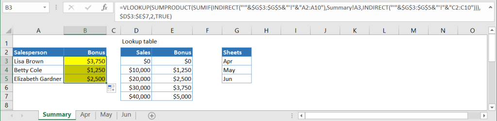
Congratulations! You’ve calculated the bonus for each salesperson across multiple sheets by using three functions: SUMIF, SUMPRODUCT, and VLOOKUP!
Load data to Excel and transform
We’ve shown you how to use Excel SUMIF and VLOOKUP together in one formula. And we hope you found the examples helpful for figuring out when they complement each other best.
Check out also another time saving combination of SUM and VLOOKUP functions.
The next time you need to pull and consolidate data from cloud apps in Excel, use Coupler.io! It not only automates data export on a schedule, but also allows you to blend, aggregate, and organize your data ?
