Calculating the sum of values across multiple columns is a common problem in Excel. The SUM function will work in most cases. However, what if you have many rows and need to quickly find a particular row to sum up related values in different fields? In that case, the combination of SUM and VLOOKUP is a great time saver!
This blog post focuses on several examples of using Excel VLOOKUP and SUM in one formula. It also covers how to write these functions in VBA code.
How to use SUM and VLOOKUP together in Excel
In most situations, the combination of SUM and VLOOKUP functions in Excel is useful when calculating the total of matching values in multiple columns. For example, to find the total purchase of a specific customer across 12 months, as the following screenshot shows:
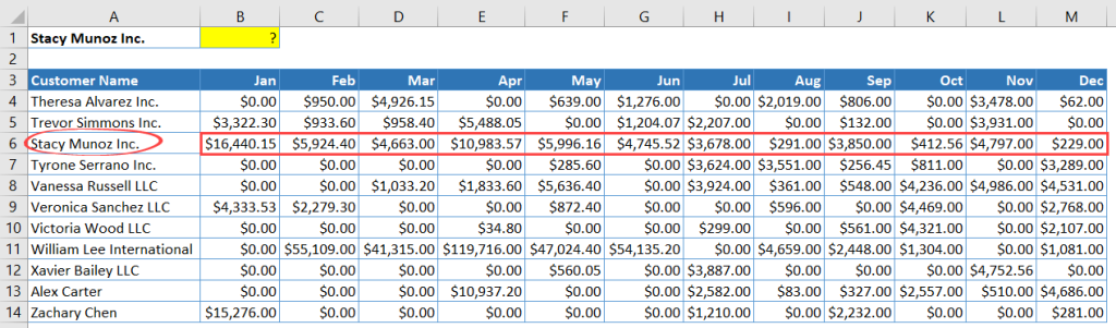
You may be wondering if you could simply use the SUM function. Why not just use =SUM(B6:M6)? Well, of course you can! But what if you want to determine how much someone spends by changing the value in A1? In this case, you would need to use a combination of VLOOKUP and SUM instead.
This is the common combination formula for SUM + VLOOKUP:
=SUM(VLOOKUP(lookup_value, table_array, col_index_num, [match_type])The useful part of this combination is when you use an array of numbers in the third parameter of VLOOKUP, for example:
=SUM(VLOOKUP(lookup_value, table_array, {2,3,4}, [match_type])Why? Because you won’t really need the SUM function if your VLOOKUP only returns one column — unless you use multiple VLOOKUPs inside a SUM.
If you’re looking for how to use VLOOKUP and SUMIF together, check out our article on that: Excel SUMIF with VLOOKUP Formula Examples.
Examples of Excel SUM and VLOOKUP to sum all matches values in multiple columns
Let’s explore some examples of using VLOOKUP and SUM functions together in one formula in Excel.
#1: Excel VLOOKUP and SUM multiple columns
In the example below, we use Excel VLOOKUP and SUM to calculate the total sales of “Barberton Daisy” for 6 months, from January to June.
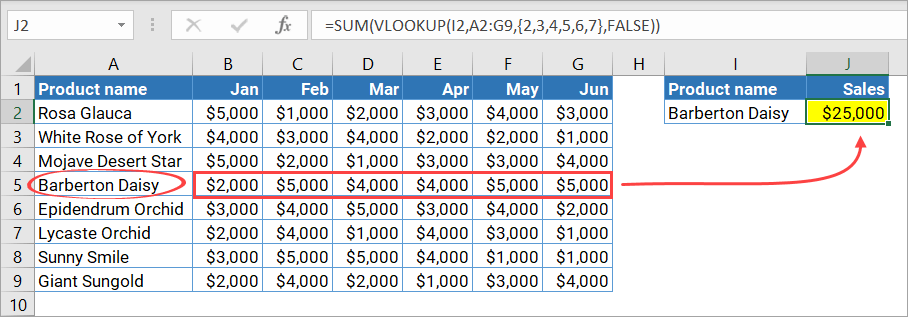
Here is the formula in J2, as you can see in the screenshot above:
=SUM(VLOOKUP(I2,A2:G9,{2,3,4,5,6,7},FALSE))
Explanation:
The VLOOKUP formula looks up for “Barberton Daisy” (the value in I2) in the first column of range A2:G9. Then, it returns values from the 2nd, 3rd, … , 7th column of the range (column B-G). After the VLOOKUP function has been executed, it returns an array of values with these elements: {2000,5000,4000,4000,5000,5000}. You can then use this result in a SUM calculation. The formula will look like this below, which equals 25000.
=SUM({2000,5000,4000,4000,5000,5000})
#2: Excel VLOOKUP and SUM: Use data from another sheet
What if you want to do the calculation from another sheet? Let’s say you have two worksheets, Summary and Sheet1, and in the Summary sheet you want the total sum of per-product sales for data on Sheet1.
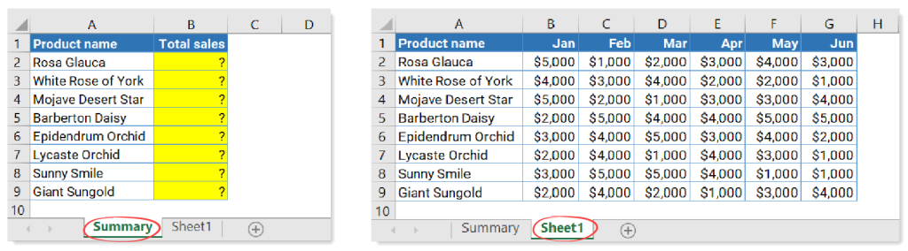
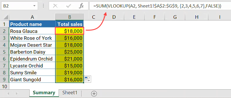
In this case, you can use the following combination of VLOOKUP and SUM in B2, then apply it down to B9.
=SUM(VLOOKUP(A2,Sheet1!$A$2:$G$9,{2,3,4,5,6,7},FALSE))
Explanation:
As you can see, to access the lookup table, the formula uses Sheet1!$A$2:$G$9 instead of simply A2:G9. This is because the lookup table is located in Sheet1, which is on a different sheet from where we wrote the formula. You need to apply the formula to B3-B9 so by using an absolute reference to the lookup table, you can ensure that its range doesn’t change in these cells.
#3: Excel VLOOKUP and SUM matches values across multiple sheets
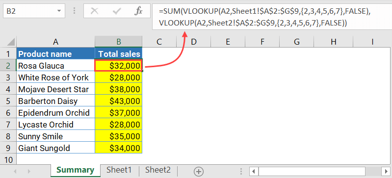
Now, suppose you have the following spreadsheet containing sales data. It has three sheets: Summary, Sheet1, and Sheet2. You want to calculate the total sales in Sheet1 and Sheet2 for each product. Then, put the result in the Summary sheet.
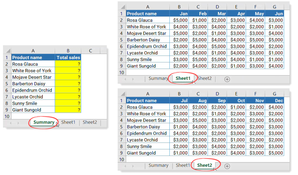
In this case, you can simply use two VLOOKUP functions inside a SUM. Here’s the formula in B2 — and you need to copy it down to B9:
=SUM(VLOOKUP(A2,Sheet1!$A$2:$G$9,{2,3,4,5,6,7},FALSE),VLOOKUP(A2,Sheet2!$A$2:$G$9,{2,3,4,5,6,7},FALSE))
Explanation:
The first VLOOKUP gets monthly sales in Sheet1 across January-June. The second VLOOKUP gets the monthly sales in Sheet2 across July-December. Finally, the SUM function adds the results from both VLOOKUPs.
#4: Excel VLOOKUP and SUM with array formula
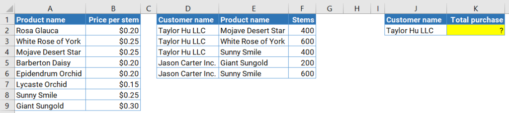
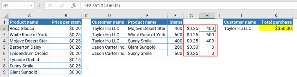
Suppose you have the following spreadsheet that contains two tables. The first table lists product names (flowers) and their price per stem. The second table contains customer names, product names, and total stems purchased. Now, you want to calculate how much the total purchase is for a given customer in J2.
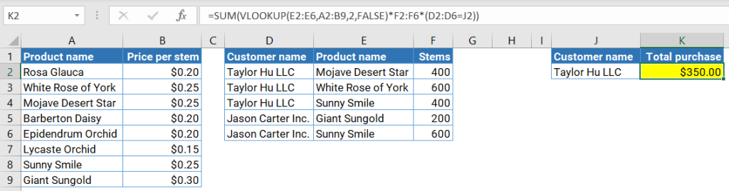
If you use the latest Microsoft 365 upgrade, you can use the combination of SUM and VLOOKUP, as shown in the below screenshot. Note: it’s an array formula, however, pressing Ctrl+Shift+Enter to wrap the formula in curly braces is no longer necessary in the current version of Excel.
=SUM(VLOOKUP(E2:E6,A2:B9,2,FALSE)*F2:F6*(D2:D6=J2))
Explanation:
VLOOKUP(E2:E6,A2:B9,2,FALSE)is used to return an array of prices per product in range E2:E6. If you copy-paste the formula in a cell, such as G2, it will spill multiple results as follows:
F2:F6*(D2:D6=J2)returns the number of stems from column F multiplied by 1 if the customer name in column D equals “Taylor Hu LLC“, otherwise it is multiplied by 0. Here is the result if we copy-paste this part in cell H2:
- Finally, the whole formula is like multiplying the results in range G2:G6 with H2:H6, which returns $350.
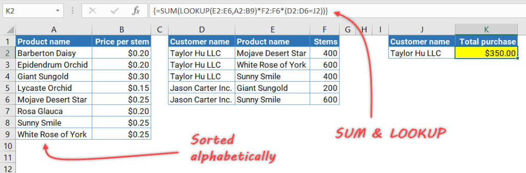
Note: You can’t use the above solution if you use an older version of Excel, for example, Excel 2010. As an alternative, you can use the SUM and LOOKUP functions instead. Keep in mind that the lookup table in the range A2:B9 needs to be sorted alphabetically if you are using the LOOKUP function. Additionally, you’ll have to press Ctrl+Shift+Enter to make the array formula work. Here’s how the final formula should look if you use this method:
Examples of what VLOOKUP and SUM can’t do: Sum all matches values in multiple rows
#5: Excel VLOOKUP and SUM: Lookup value in duplicate rows
With the following data, suppose you want to calculate how many sales were generated by Orchid for six months, from January to June.
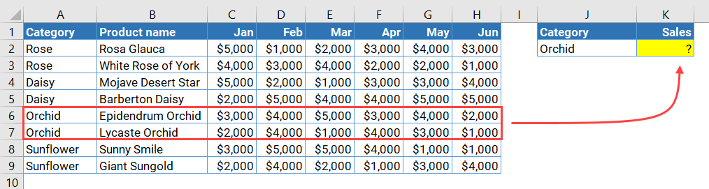
See that you have duplicate rows for Orchid. In this case, you can’t use the combination of Excel SUM and VLOOKUP. Using VLOOKUP to search for “Orchid” always returns the first matching value only.
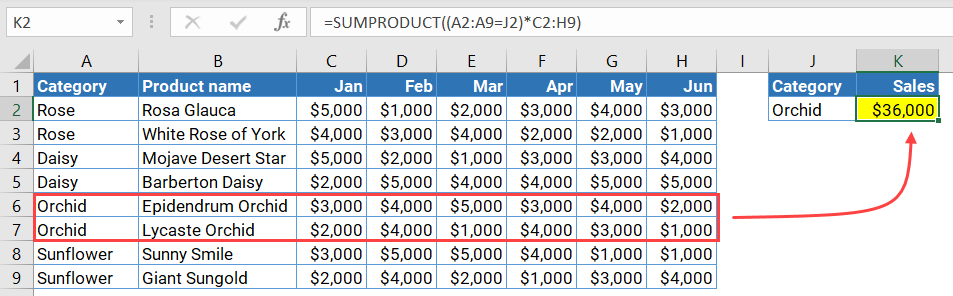
One alternative is by using the SUMPRODUCT function, as follows:
=SUMPRODUCT((A2:A9=J2)*C2:H9)
Explanation:
The first expression A2:A9=J2 checks the range A2:A9 and returns an array of TRUE FALSE. If any cell equals “Orchid“, it will return TRUE, otherwise it returns FALSE:
{FALSE;FALSE;FALSE;FALSE;TRUE;TRUE;FALSE;FALSE}
The result above is then multiplied by the values in range C2:H9 and creates the following array:
{0,0,0,0,0,0;0,0,0,0,0,0;0,0,0,0,0,0;0,0,0,0,0,0;3000,4000,5000,3000,4000,2000;2000,4000,1000,4000,3000,1000;0,0,0,0,0,0;0,0,0,0,0,0}
Finally, the SUMPRODUCT calculates the total of all the elements in the above array and returns 36000.
#6: Excel VLOOKUP and SUM values between two dates
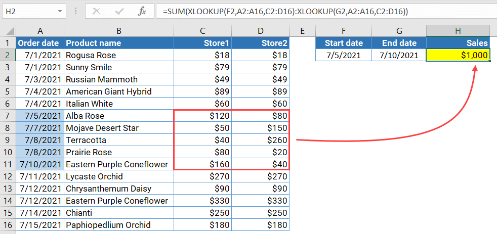
In the example below, suppose you want to sum up the sales of multiple records by order date. There are two columns and a few rows that you need to sum. Notice that there are even rows with the same order dates.
A combination of SUM and VLOOKUP won’t be able to solve this problem. One alternative is to use the SUM function with two nested XLOOKUP functions, as shown in the following formula:
=SUM(XLOOKUP(F2,A2:A16,C2:D16):XLOOKUP(G2,A2:A16,C2:D16))
Please note that the XLOOKUP function only works in Microsoft 365 and Excel for the web (Excel Online version). Also, see our guide on XLOOKUP: Excel XLOOKUP function.
Explanation:
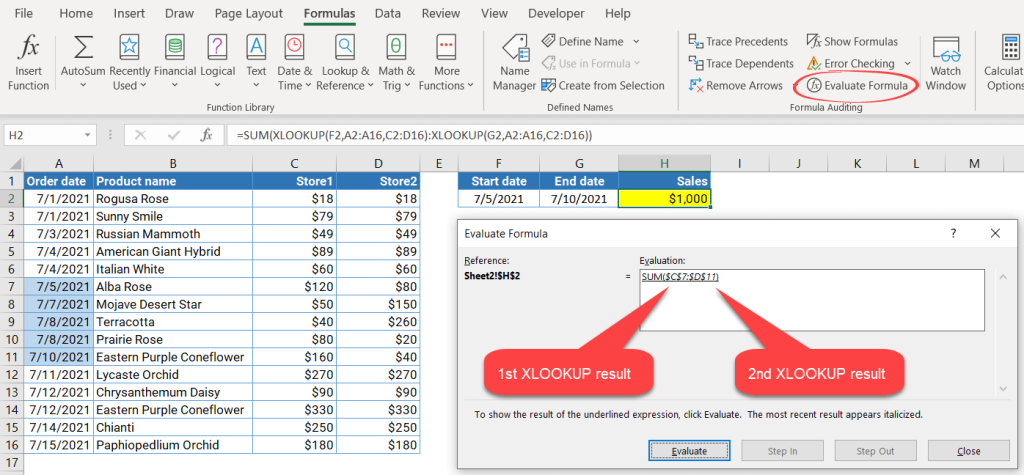
The formula uses two nested XLOOKUP functions to create a range dynamically by returning the starting cell and ending cell on either side of the colon range operator. The first XLOOKUP returns the first cell reference in the range, while the second XLOOKUP returns the last cell reference in the range. After the nested functions have been executed, the SUM function would look like this:
=SUM(C7:D11)
Tip: You can use the Evaluate Formula dialog box to observe how the XLOOKUP functions are being evaluated and their return result. To do this, first, select the cell that we want to evaluate, in this case H2. Then, in the Formula tab, click on the Evaluate Formula button in the Formula Auditing group. A dialog box will appear, allowing you to evaluate the formula, expression by expression.
Excel VBA: SUM + VLOOKUP
You may want to use SUM and VLOOKUP in VBA, for example, when you need to do it as a part of a larger task. Let’s say, every week you need to pull sales data from several external systems into Excel, do a bit of cleanup, and send a report in PDF related to a certain product. Additionally, in a specific part of that report, you need to do a calculation using SUM and VLOOKUP.
Tip: You can pull data from external sources into Excel without coding by using an integration tool such as Coupler.io. With it, you can save your time by importing data from different sources like Airtable, Jira, Shopify, HubSpot, and many others into Excel. The best part? You can even set automatic data refresh on the schedule you want!

Check out the complete list of Coupler.io integration with Excel.
How to write a formula of VLOOKUP + SUM in Excel VBA
Both SUM and VLOOKUP are worksheet functions in Excel. You can use them in VBA by typing WorksheetFunction.<function_name>. Here are the syntaxes of both functions:
- The SUM’s syntax in VBA
WorksheetFunction.Sum(Number1,Number2,...,Number30)
Where Number1,Number2,...,Number30 are the values that you want to sum. You can have up to 30 arguments.
- The VLOOKUP’s syntax in VBA
WorksheetFunction.Vlookup(lookup_value, table_array, col_index_number, [match_type])
The syntax is similar compared to when you’re using it in a cell, and the number of arguments is also the same. However, in VBA, when you pass an array in the third argument, the VLOOKUP will return the result for the first element only. Thus, you need to do the VLOOKUP in a loop if you want to return multiple results.
How to sum up numbers in multiple columns using VLOOKUP + SUM in Excel VBA
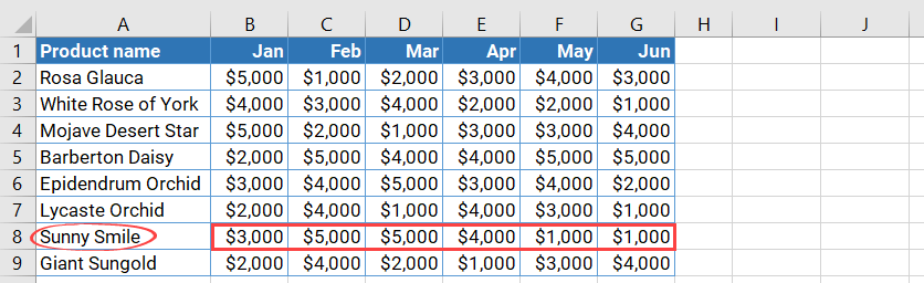
Now, let’s look at the example below. Suppose you have the following table and want to sum the total sales generated by “Sunny Smile” using VBA.
To do that, follow the steps below:
Step 1: Press Alt+F11 to open the Visual Basic Editor (VBE).
Step 2: Create a new Sub, for example, “MySumVlookup“.
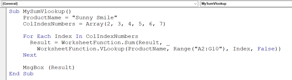
Sub MySumVlookup()
    ProductName = "Sunny Smile"
    ColIndexNumbers = Array(2, 3, 4, 5, 6, 7)

    For Each Index In ColIndexNumbers
      Result = WorksheetFunction.Sum(Result, _
        WorksheetFunction.VLookup(ProductName, Range("A2:G10"), Index, False))
    Next

    MsgBox (Result)
End Sub
Screenshot:
Explanation:
We declared a variable called ColIndexNumbers that contains the indexes of columns in range A2:G10 that we want to sum. The code loops through each element in the array and in each loop it performs VLOOKUP and adds the result into the Result variable. Finally, the code returns the end result in a message box.
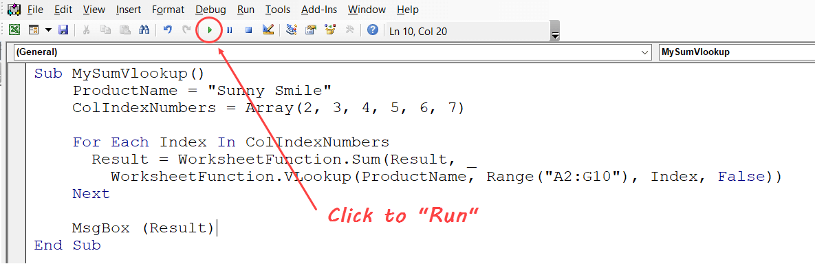
Step 3: Run the Sub by pressing the green triangle button in the toolbar.
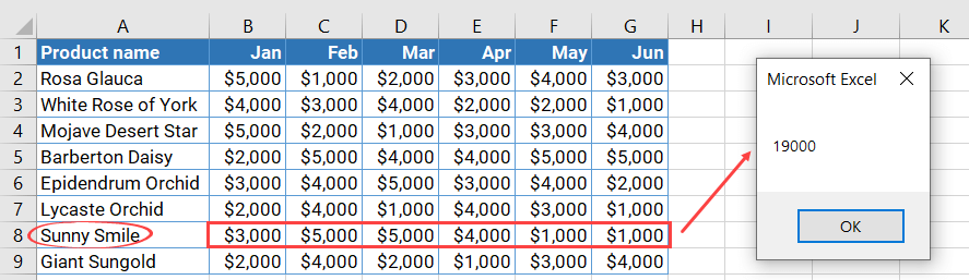
You will see a message box showing the result, as follows:
When your Excel VLOOKUP + SUM is not working
So, you’re using a combination of SUM and VLOOKUP functions in Excel but running into a problem? Check for the following things:
- Ensure your data has the correct format, especially if you imported them from other systems. Numbers are often mistaken for text and need to be converted into “actual” numbers. Similarly, dates can sometimes be exported as text and get mixed up. Make sure you double-check any date values before moving on with the rest of your analysis.
- Double-check each parameter value of your VLOOKUP function. You might have inputted a wrong lookup value, used approximate matches when you intended to search for an exact match, etc. For the most common errors, see this list: VLOOKUP formula is not working.
- If you need to apply a combination of both functions in multiple cells (like in example #2), use an absolute reference for your lookup table. This will ensure that the range is fixed and doesn’t change! Just press F4 after entering a cell reference; Excel automatically makes it into an absolute reference.
- If you use any Excel version older than Microsoft 365, always press Ctrl+Shift+Enter when using array formulas inside the SUM and lookup functions. This will wrap your formula in curly braces and return the correct result.
Wrapping up
We’ve covered various examples of using Excel VLOOKUP and SUM together. You’ve seen the different scenarios where this combination can be helpful, as well as some limitations it has with summing data in multiple rows.
In addition, if you’ve been struggling with how to pull data from external systems, such as Jira, Shopify, WordPress, etc., or even JSON formatted data from REST APIs into Excel, try Coupler.io. Take advantage of this integration tool to do the imports with ease. You don’t even need to write any VBA code. ?
