In Google Sheets, there is a wonderful function called IMPORTRANGE. It allows you to link a specific range of cells from one spreadsheet to another. And how to link Excel worksheets? Let’s find out whether you can use IMPORTRANGE in Excel or use other functionality to do this.
Is there IMPORTRANGE in Excel?
There are many functions in Excel, such as VLOOKUP Excel or SUMIF Excel. However, there is no Excel IMPORTRANGE function.
At the same time, Excel provides a similar to IMPORTRANGE functionality for linking a data range from a separate spreadsheet. This can be done either by copying and pasting a data range or by using a formula bar.
What is the Excel version of IMPORTRANGE?
In Excel Online, the IMPORTRANGE functionality is called Workbook Links. I’ll cover the details of Workbook Links later.
In Excel desktop, it has no explicit name but is implemented via the Paste Link option.
The implementation of an Excel IMPORTRANGE equiv depends on the Excel app you use (365/Online or desktop app). Let’s discuss each way separately.
IMPORTRANGE/Workbook Links alternative for Excel
In essence, both Excel Workbook Links and IMPORTRANGE synchronize data between two sheets. So, if the data in the source sheet changes, these changes are visible in the destination sheet. And this could be an issue if, for some reason, the data in the source sheet was corrupted or the file was broken. As a result, the valuable information disappears in both sheets. With the Excel integrations by Coupler.io, you won’t have this risk.
Using the Coupler.io web app or add-in for Excel, you can also connect workbooks. However, unlike Workbook Links or IMPORTRANGE, the Excel integration by Coupler.io imports data from one sheet to another. So, if the source workbook is not accessible for some reason, you will still have your data set in the destination workbook.
Connecting Excel workbooks with Coupler.io only takes three steps and does not require any formulas. All you need to do is click Proceed in the form below:
You’ll be offered to create a Coupler.io account for free.
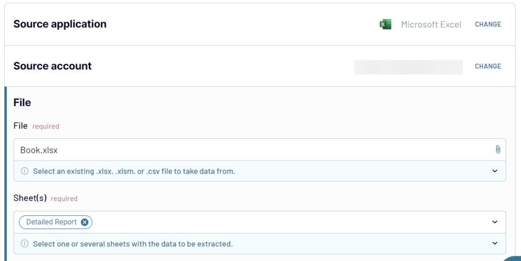
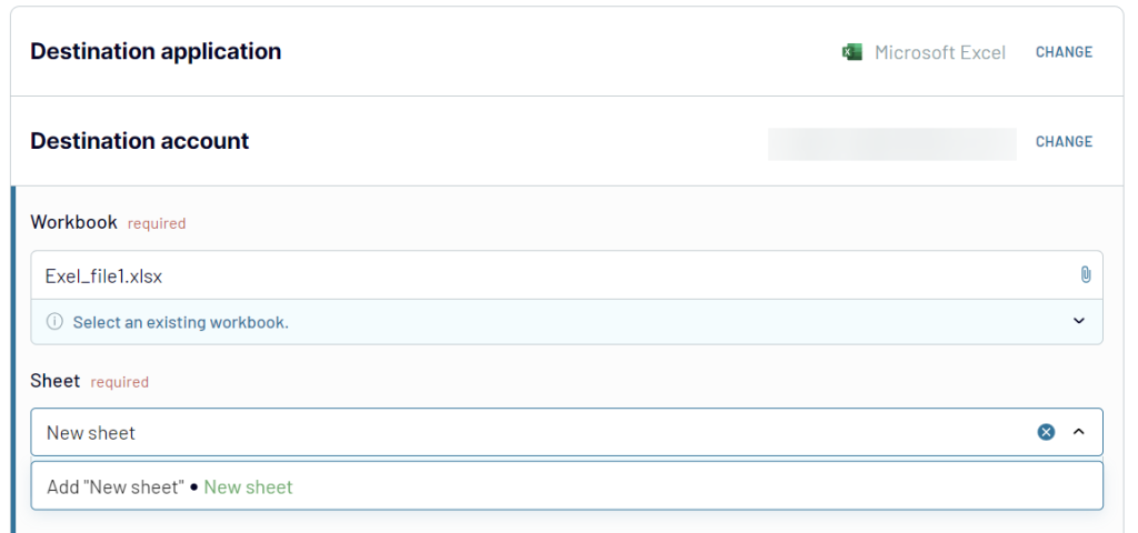
- Then, in your OneDrive folder, select the Excel workbook and sheet(s) to get data from.
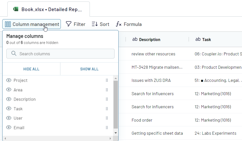
- Preview and transform the data, if needed, before loading it to the destination Excel workbook.
- In your OneDrive folder, select the Excel workbook and sheet to load data.
This is a high-level flow but you can also enjoy a number of optional parameters and features:
- Select multiple sheets to concatenate data from them into one master view.
- Join data from multiple worksheets using a key column.
- Specify a range, not an entire sheet, to import.
- Specify the first cell to load data to.
- Change the import mode from replace to append. With the replace mode, all the new data will replace the previously imported records. With the append mode, the newly imported records will be added under the previously imported ones.
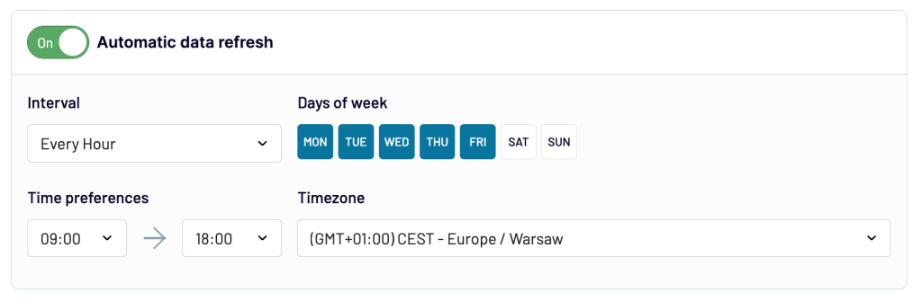
The icing on the cake is the automatic data refresh. Coupler.io allows you to automate the import of data on a custom frequency from once a month to every 15 minutes. To do this, toggle on the Automatic data refresh and configure the schedule for your data import.
From the moment you click Run importer, the data flow between the selected Excel files will be automated. You will be sure to have up-to-date information without spending a minute on manual data transfer. Actually, Coupler.io will save you up to 60% of your time – this is quite a significant improvement in your reporting and analytics.
In addition to that, I have to mention that Coupler.io is not limited to Excel integrations. You can load data from business apps to Excel, or connect your Excel files to other destinations like Google Sheets, BigQuery, or Looker Studio. You should definitely try it!
How to use IMPORTRANGE equivalent for Excel desktop
I promised to share the details of using Workbook Links in Excel. Let’s start with how this works for desktop Excel.
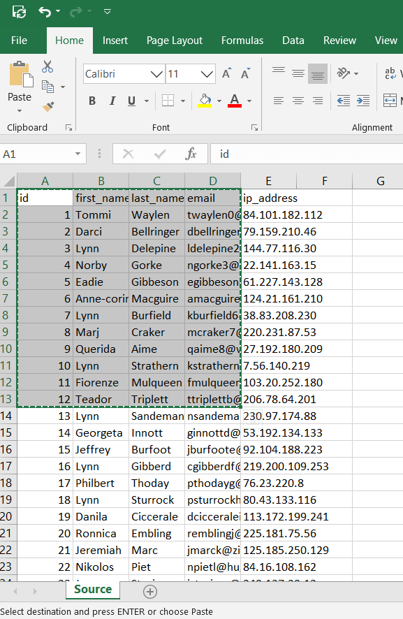
Open both a source and a destination Excel spreadsheet. Select a range of cells in the source spreadsheet and copy them: you can use either Ctrl+C or right-click => Copy.
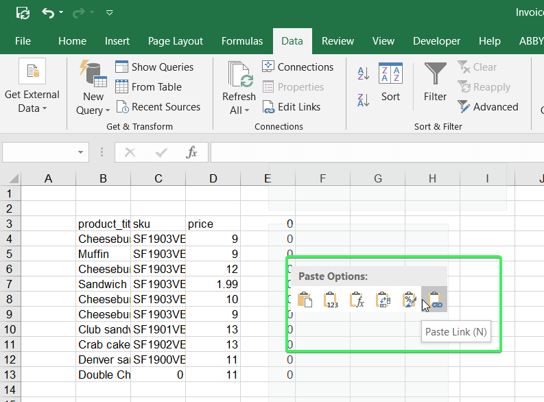
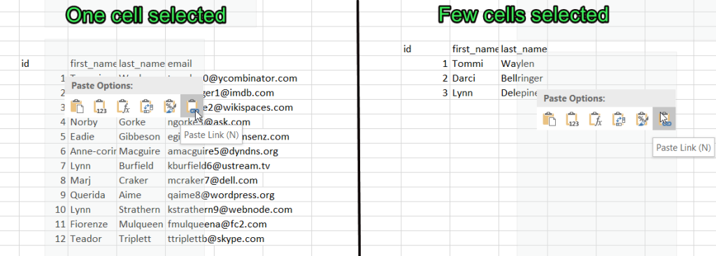
Go to your destination spreadsheet, select either one cell to import the entire range or a range of cells to only populate the selected cells. Then right-click and select Paste Link.
You can expand the imported range by simply dragging the cross as follows:
Now if you change some values of the imported range in the source file, the values in the destination spreadsheet will be updated as well.
This method works well if your source and destination spreadsheets are open. When you need to import a range from an Excel workbook that is not open, use the formula bar method.
Excel IMPORTRANGE formula using the formula bar in desktop app
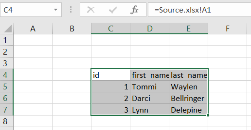
First of all, an important note: If your source workbook only has one worksheet with the same name as the workbook, the imported range reference will look as follows in the formula bar:
={workbook-name}.xlsx!{first-cell}For example:
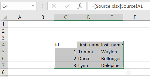
However, if the names of the source workbook and worksheets differ, or the workbook has multiple worksheets, the imported range reference will look as follows in the formula bar:
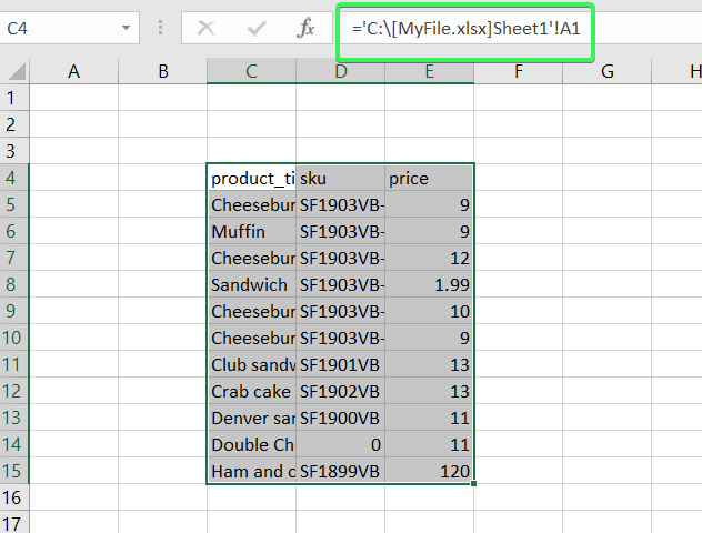
=[{workbook-name}.xlsx]{worksheet-name}!{first-cell}For example:
When you close the source workbook, the imported range reference transforms in the following way:
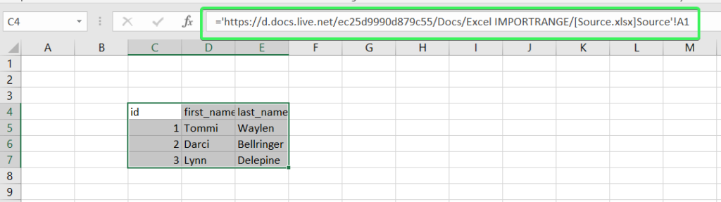
So, it’s attached with a path to the file on your device. In our case, the path is to the OneDrive storage folder. However, you can also encounter more regular paths like this one:
This is the boilerplate you can use to import data from any Excel file on your device:
='{path-to-file}/[{workbook-name}.xlsx]{worksheet-name}'!{first-cell}
Note: you can use either slash or backslash depending on which type is used in the path to your file.
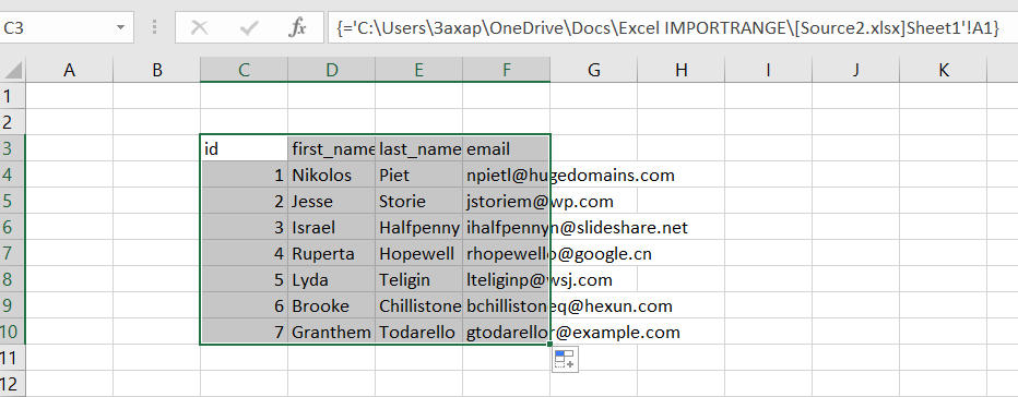
For example, we need to import data from Sheet1 of a source file named Source2.xlsx stored in the OneDrive folder. In the example above, our reference to this folder looked as follows:
https://d.docs.live.net/ec25d9990d879c55/Docs/Excel IMPORTRANGE/
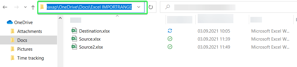
But it’s okay if you take a regular path, which you can find in the file explorer like this:
C:\Users\?????\OneDrive\Docs\Excel IMPORTRANGE
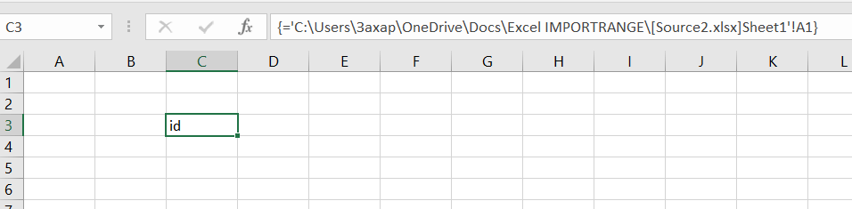
Insert this path string to the Excel IMPORTRANGE equivalent formula and add other variables: {workbook-name}, {worksheet-name}, and {first-cell}. Here is what we’ve got:
='C:\Users\?????\OneDrive\Docs\Excel IMPORTRANGE\[Source2]Sheet1'!A1
Select a cell, insert this formula to the formula bar and press Ctrl+Shift+Enter.
Now you can expand the range by dragging the cell vertically or horizontally.
If you want to import an exact range at once, specify the range instead of the first cell in your formula. Then select the range in the destination sheet, insert the formula to the formula bar, and press Ctrl+Shift+Enter. Here is an example:
='C:\Users\?????\OneDrive\Docs\Excel IMPORTRANGE\[Source2]Sheet1'!A1:C10
Note: if you select the number of cells greater than the number of cell in the range to import, you’ll get
#N/Afor the cell beyond the range.
Workbook links – Excel IMPORTRANGE from different worksheet online
Now you have an understanding of how IMPORTRANGE functionality on Microsoft Excel desktop works. However, Excel Online, as well as Excel 365, has some differences in use. Let’s explore how Workbook Links works.
Open the files you already know, Source.xlsx and Destination.xlsx, in Excel Online. Select and copy a range in the source file, go to the destination file, select a cell, right-click, and choose Link as a paste option.
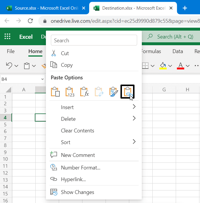
The cells will be populated with the values from the source spreadsheet.
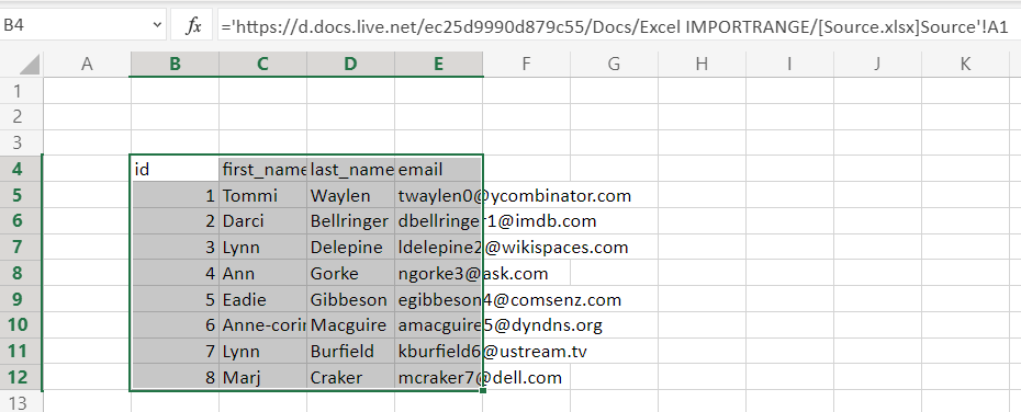
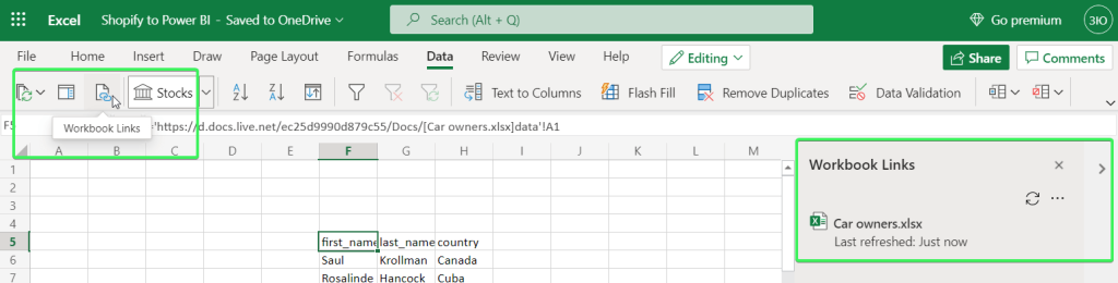
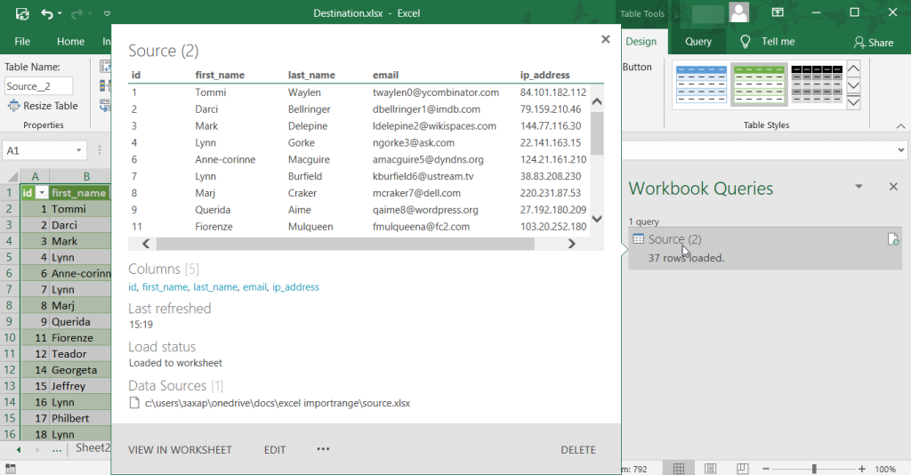
The main difference here is that the imported data won’t be refreshed automatically until you enable this. To do this, go to the Data menu => Workbook Links.
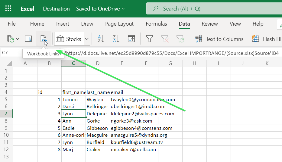
On the pop-up panel on the right, click the three dots and check the Refresh automatically checkbox for the linked workbook.
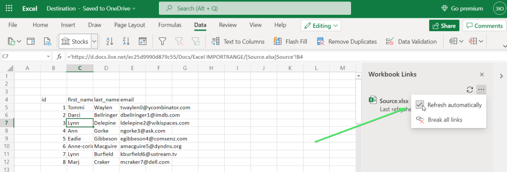
Now the imported range will be refreshed automatically every 5 minutes to display any change in the source range.
Excel Workbook Links does not work
We tried to import a range from a file stored in another folder, and here is the result:
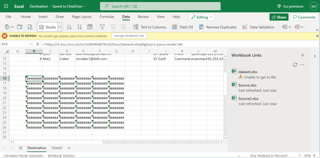
We referenced a thread on the MS Office forum regarding the same issue, but we’ve still had no luck in resolving it. The only method that worked was to put the source and destination workbooks in the same folder.
With this in mind, it’s good to have a failsafe alternative to link Excel to Excel. And there is one – Coupler.io.
IMPORTRANGE from Excel to Google Sheets and vice versa
The real IMPORTRANGE function only connects Google Sheets documents. IMPORTRANGE in Excel, Workbook Links, only connects Excel files. With Coupler.io, you can mix those functionalities and synchronize data between an Excel workbook and a Google spreadsheet.
For example, to import a range from an Excel spreadsheet to Google Sheets, you need to choose Excel as a source app and select the file to get data from. As a destination app, choose Google Sheets, and select the file to load data to.
Excel IMPORTRANGE FAQs
The two most popular spreadsheet apps, Google Sheets and Excel, have a large influence on each other’s progress. IMPORTRANGE is a case in point because it’s a Google Sheets function that is not available in Excel. Nevertheless, many users keep using the term Excel IMPORTRANGE to name Workbook Links…or they just dream about a day when the Microsoft team releases this function. 🙂 Anyway, we collected a few questions associated with this and hope you’ll find it useful.
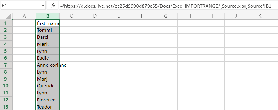
Excel IMPORTRANGE function for a whole column
Everything works as usual. To import an entire column from one workbook to another, just select the column (click the column index letter), copy it, and paste as link into the destination workbook.
How to use Excel IMPORTRANGE to get data with formatting?
IMPORTRANGE in Google Sheets, Workbook Links in Excel, as well as Coupler.io, allow you to only import raw data without formatting.
Can I use Excel IMPORTRANGE with CONCATENATE?
In Google Sheets, you can nest IMPORTRANGE with CONCATENATE, QUERY, and many other functions. For example, check out our IMPORTRANGE+QUERY tutorial.
However, in Excel, there is no IMPORTRANGE function, so it’s impossible to do.
Excel IMPORTRANGE to import cells with text only
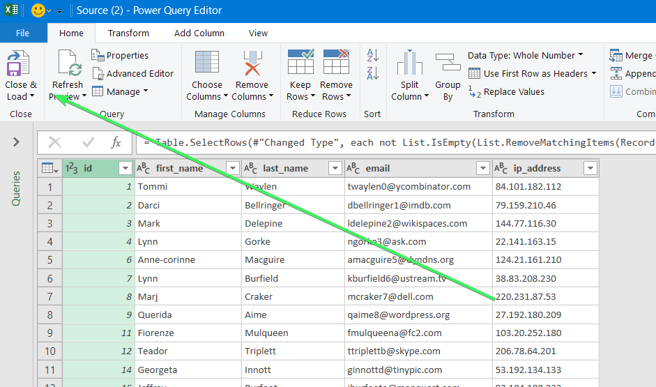
Unfortunately, Workbook Links does not let you set conditions for the ranges you import. However, you can use the Excel Power Query to do the job. For example, our data set that we need to import contains empty rows:
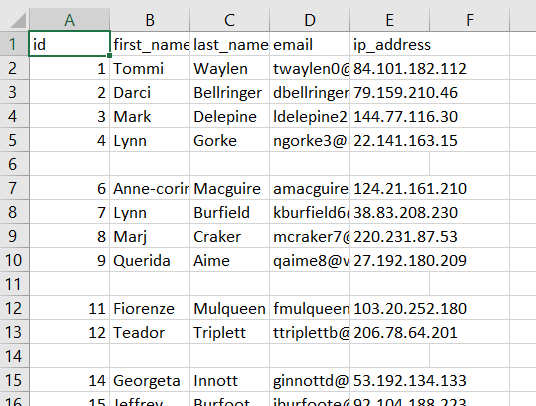
We can set a condition to ignore them for our import.
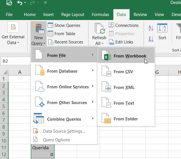
- Go to the Data menu => New Query => From File => From Workbook
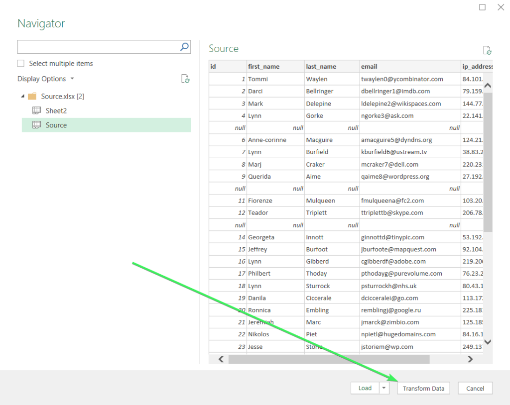
- Select your source workbook. In the Navigation window, select a sheet and click “Transform Data“.
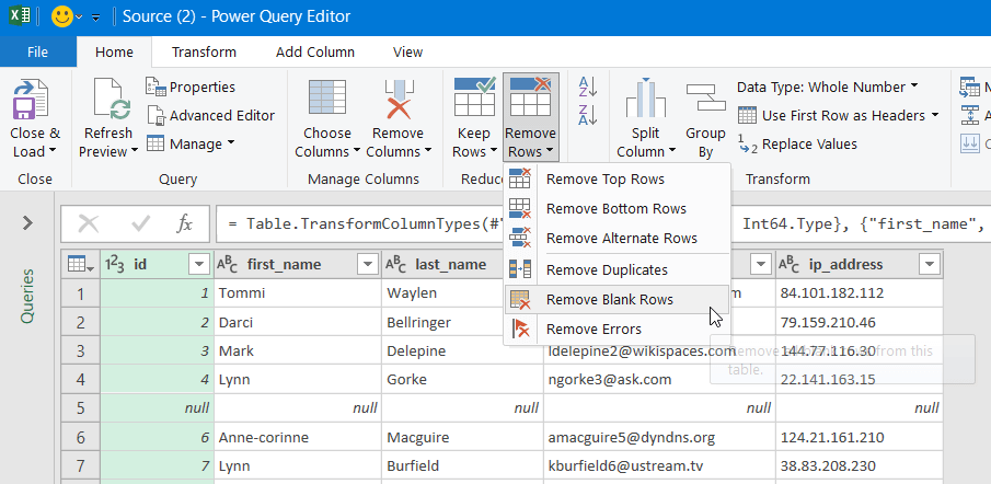
- This will bring you to the Power Query Editor, where you can add or remove columns/rows, change data types, split columns, group values by columns, and perform other sorts of data manipulation. What we need is to remove blank rows. There is a dedicated button for this on the ribbon menu: Remove Rows => Remove Blank Rows.
- All blank rows have been removed. Now you can Close & Load your data range. Click the respective button.
- Welcome your data range into your sheet. Now the source sheet is connected to your destination sheet, and the queried data range will be refreshed automatically every 5 minutes, or you can do this manually.
IMPORTRANGE, Workbook Links, or Coupler.io
Who’s going to win this race? Only Coupler.io is designed for both Excel and Google Sheets users and provides them with a scheduled data refresh, support for multiple sources and destinations, and many other cool features.
IMPORTRANGE is only available for Google Sheets users. It’s a good function, although it is known for its errors, which we’ve covered in Why IMPORTRANGE Is Not Working: Errors and Fixes.
Workbook Links, looks a bit plain and straightforward compared to its competitors. The keyword “excel importrange” is highly requested in Google search results, which means that Excel users need this function instead of WL. Ugly truth.
So, make your choice for importing data and good luck with it!

Automate data export with Coupler.io
Get started for free