VLOOKUP Google Sheets Explained: How to Search Data Vertically in Spreadsheets

How do you learn the status of your flight on the flight board in the airport? First, complete a vertical lookup to find the necessary flight number, for example, AC5704. After doing so, shift your eyes to the right to find the respective value in the Status column.

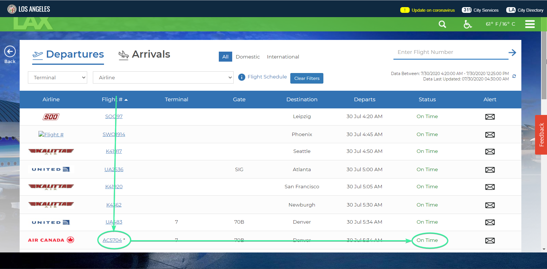
The VLOOKUP function in Google Sheets works in a similar way as it searches vertically for the specified value and returns matching data from the row. Read this tutorial to explore the basic and advanced capabilities of VLOOKUP.

If you prefer watching to reading, check out this 3-minute video tutorial explaining the basics of the VLOOKUP Google Sheets function.

Understanding vertical lookup or VLOOKUP in Google Sheets for dummies

VLOOKUP formula syntax

=VLOOKUP(search-key, range, column-index, [sorted/not-sorted])

• search-key – specify what you’re going to look up. This can be either a text string ("Text"), number (5), date (2020-01-02), or a cell absolute reference (A2). Text to search must be entered in quotes only.
• range – specify the data range on any sheet to look up. 
• column-index – specify the number of the column in the lookup range from which the matching value will be returned. The index of the first column of the range is always 1.
• [sorted/not-sorted] – specify whether the lookup column is sorted from A to Z (TRUE) or not (FALSE). It is an optional parameter with TRUE as the default value.

VLOOKUP always returns the first value found, even if the looked up column contains two or more values matching the search-key.

How to VLOOKUP in Google Sheets – formula example

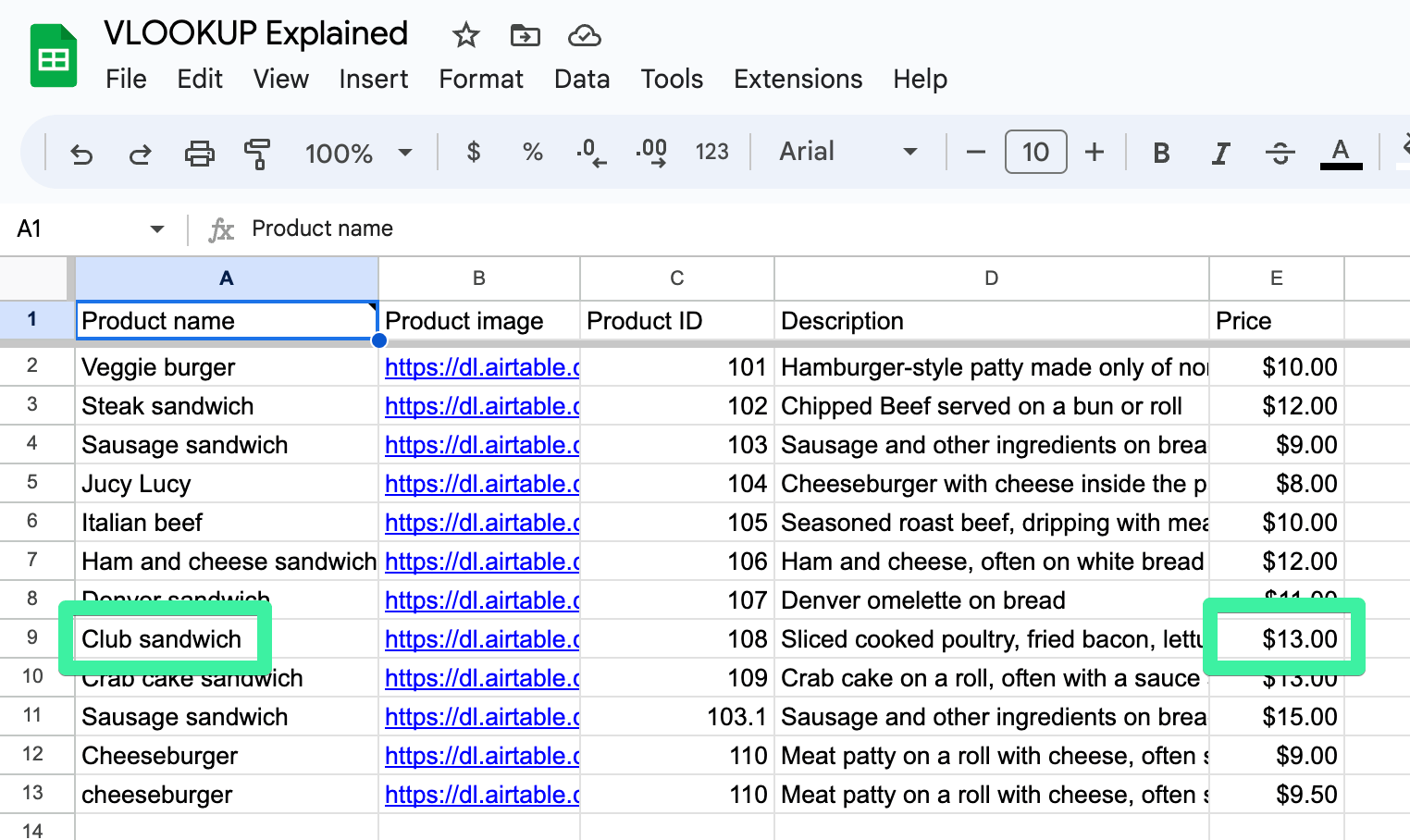
Let’s extract the price of the Club Sandwich from the following data set.

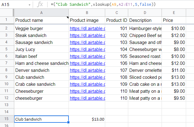
Here is the VLOOKUP formula to do this:

={"Club Sandwich",
   vlookup(
      A9,
      A2:E11,
      5,
      false
   )
}

• {"Club Sandwich"...} – this will add the name (Club Sandwich) to the cell to the left of the value returned by the VLOOKUP formula
• A9 – the search-key we’re looking up
• A2:E11 – the data range 
• 5 – the column number (index number) of the data range to look up
• false – the lookup column is not sorted

That’s the basics. Now let’s dive deeper into how you can use VLOOKUP.

VLOOKUP function in Google Sheets – Cheat Sheet 

If you are not a novice to VLOOKUP and merely need to brush up your skills, check out the following VLOOKUP cheat sheet.

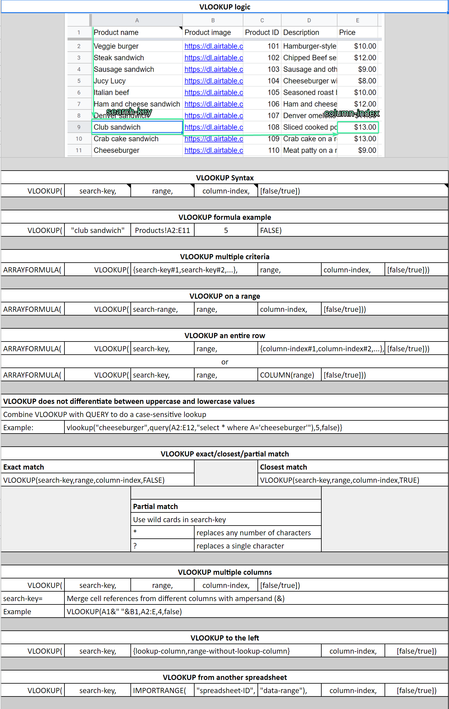
VLOOKUP Cheat Sheet in Google Sheets

How to do VLOOKUP in Google Sheets – tutorial with examples

Before we start exploring the VLOOKUP function in Google Sheets, let’s first load some sample data into our spreadsheet. We’ll then use this data for demonstration.

• To load data into a spreadsheet, we’ve used one of the Google Sheets integrations provided by Coupler.io. This is a handy platform for importing data to Google Sheets, Excel, BigQuery, and Looker Studio. It can pull data from 70+ different apps, such as Airtable, Pipedrive, QuickBooks, and many others. The platform lets you combine data from different sources, transform it, and bring it to the desired destination in a fully automated manner, on the schedule you choose. In addition, no tech skills are required to create these automations, so anyone can do it.  
• See the full list of data sources that you can export to Google Sheets. We definitely recommend giving it a try as it makes working with Google Sheets much easier.

To export data, sign up with your Google account – this literally takes seconds. Then, select the app you want to extract data from, choose Google Sheets as a destination, and set up an automated connection following further instructions.

• If you need more details on this, you can review this guide.
• In several minutes, your dataset will be imported to Google Sheets, and we are ready to dive into the details of using the VLOOKUP function.

1. How to VLOOKUP for the exact or closest match

• For an exact match, specify FALSE as the [sorted/not-sorted] parameter. It’s the recommended value.
• For the approximate match, specify TRUE as the [sorted/not-sorted] parameter.

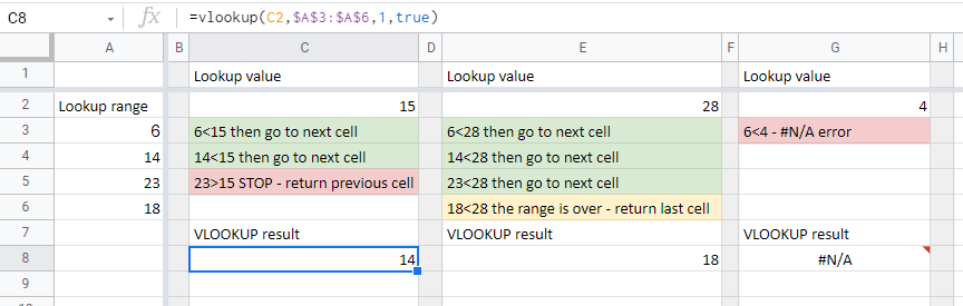
1.1 The logic of VLOOKUP with TRUE (sorted parameter) to find the closest match

If you specify TRUE as the last parameter in your VLOOKUP formula, it will search for the exact match first. If failed, function searches cell by cell for the closest match that is less than or equal to the search-key. If the search-key is less than the value in the first cell to look up, the formula will return an #N/A Error: Did not find value '***' in VLOOKUP evaluation.

2. How to VLOOKUP for a partial match using wildcards

You can use the following wildcards with your search-key in the VLOOKUP formula:

• Asterisk (*) to take the place of any number of characters.
• Question mark (?) to take the place of any single character.
• Tilde sign (~) before an asterisk (*) or a question mark (?) to treat them as simple signs. For example, “~**” means that you’re looking for the values that start with an asterisk “*”.

In our blog post about COUNTIF and COUNTIFS functions, we’ve already explained how wildcard characters work. Let’s look at it through a hands-on example, when a search-key begins, ends, or contains a specific text.
In our data set of sandwiches, we need to find the description of the product that contains “cake” in its name. Here is how the search-key should look: "*cake*". And here is the VLOOKUP formula:

=vlookup("*cake*",A2:E,4,false)

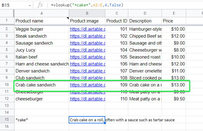
As we expected, the formula returned the description of Crab cake sandwich. In a similar manner, you can vertically look up criteria that begin or end with a particular text.

3. Google Sheets VLOOKUP multiple columns

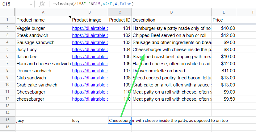
You can also use a number of columns as a search-key. Let’s say cell A1 contains ‘jucy‘, and cell B1 contains ‘lucy‘. We need to use values from these cells as a search key (‘jucy lucy‘) in the VLOOKUP formula. For this, you can merge cells using the ampersand (&) as follows: A1&" "&B1.

Now you can nest this formula with VLOOKUP:

=vlookup(A15&" "&B15,A2:E,4,false)

Note: Read more about Merging Cells in Google Sheets.

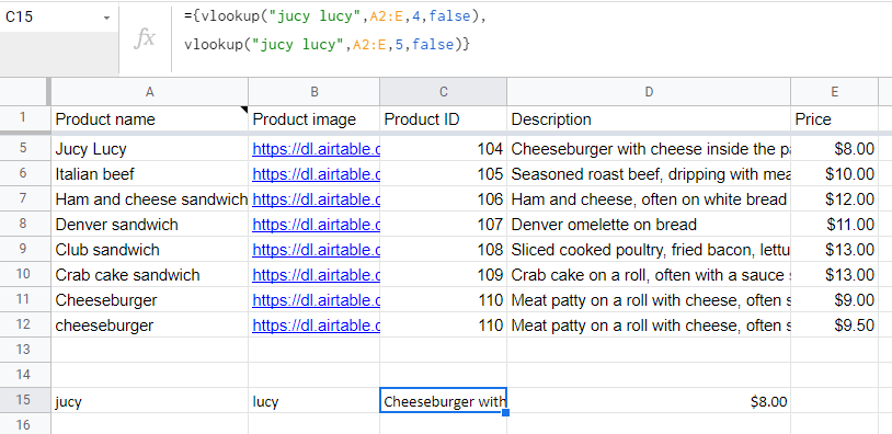
4. Google Sheets VLOOKUP multiple values

If you want to vlookup multiple values, you need to use two or more formulas wrapped in curly brackets. Each VLOOKUP formula should have a different column index:

={VLOOKUP(search-key, range, column-index-1, [sorted/not-sorted]),VLOOKUP(search-key, range, column-index-2, [sorted/not-sorted]),...}

Note: Use comma to separate VLOOKUP formulas to return the values in one row; use semicolon to return the values in one column.

For example, let’s vlookup the search key ‘jucy lucy' to return not only the description (column index 4), but also the price (column index 5). Here is the formula:

={vlookup("jucy lucy",A2:E,4,false);
vlookup("jucy lucy",A2:E,5,false)}

5. Google Sheets VLOOKUP another sheet or multiple sheets

There are no problems with using VLOOKUP for vertical search in a different sheet of your spreadsheet. For this, you need to list the sheets’ ranges using curly brackets in the range parameter. The ranges must be separated by a semicolon as follows:

=VLOOKUP(search-key, {sheet1-range;sheet2-range;sheet3-range…}, column-index, [sorted/not-sorted]) 

For example, you may have your data spread across the three sheets: Products1, Products2, and Products3. 

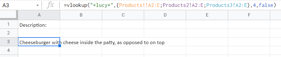
Let’s find the description of the product with a name containing “lucy”. Here is the VLOOKUP formula:

=vlookup("*lucy*",{Products1!A2:E;Products2!A2:E;Products3!A2:E},4,false)

6. How to do a case-sensitive Vlookup: QUERY and VLOOKUP 

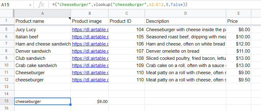
VLOOKUP does not differentiate between uppercase and lowercase values. So, with the search-key "cheeseburger", the formula will return the value that matches “Cheeseburger“, since it’s the first match when looking up:

={"cheeseburger",vlookup("cheeseburger",A2:E12,5,false)}

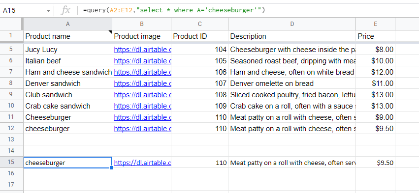
You can solve this issue by nesting VLOOKUP with QUERY since the QUERY function is case-sensitive. The following formula will filter out ‘cheeseburger‘ from the data range A2:E12:

=query(A2:E12,"select * where A='cheeseburger'")

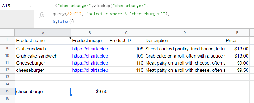
Nest this QUERY formula with the VLOOKUP formula to do a case-sensitive lookup:

={
   "cheeseburger",
    vlookup(
       "cheeseburger",
        query(A2:E12, "select * where A='cheeseburger'"),
        5,
        false
     )
}

Read our blog post to learn more about the power of the Google Sheets Query Function.

7. Google Sheets VLOOKUP multiple criteria

To Vlookup two or more search keys, nest VLOOKUP with ARRAYFORMULA as follows:

=ARRAYFORMULA(VLOOKUP({search-key#1;search-key#2;...}, range, column-index, [sorted/not-sorted])

This will return vlookup results in a column. If you want to return the results in a row, replace semicolons with commas between search keys.

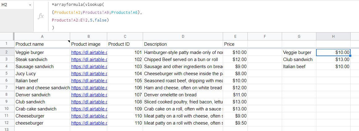
=ARRAYFORMULA(VLOOKUP({search-key#1,search-key#2,...}, range, column-index, [sorted/not-sorted])

For example, let’s vertically look up the price of ‘Veggie burger‘, ‘Club sandwich', and ‘Italian beef':

=arrayformula(
   vlookup(
      {Products!A2;Products!A9;Products!A6},
      Products!A2:E12,
      5,
      false
   )
)

Read our blog post to learn more about ARRAYFORMULA in Google Sheets.

8. Google Sheets ARRAYFORMULA VLOOKUP on a range

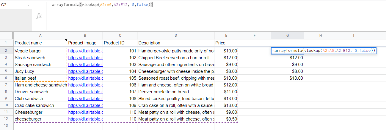
In a similar way, you can look up a data range:

=ARRAYFORMULA(VLOOKUP(search-data-range, range, column-index, [sorted/not-sorted])

For example, let’s search for the range A2:A6:

=arrayformula(vlookup(A2:A6,A2:E12, 5,false))

9. How to VLOOKUP an entire row or several values: ARRAYFORMULA and VLOOKUP

Nest VLOOKUP with ARRAYFORMULA and specify indexes of the columns you want to have data extracted from.

=ARRAYFORMULA(VLOOKUP(search-key, range, {column-index#1,column-index#2,...}, [sorted/not-sorted])

If you want to return the results in a column, replace commas with semicolons between column indexes.

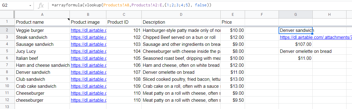
=ARRAYFORMULA(VLOOKUP(search-key, range, {column-index#1;column-index#2;...}, [sorted/not-sorted])

For example, let’s extract the entire row of ‘Denver sandwich':

=arrayformula(vlookup(Products!A8,Products!A2:E,{1;2;3;4;5}, false))

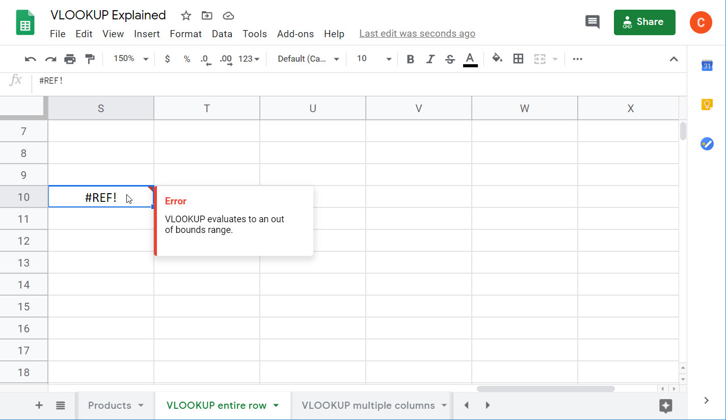
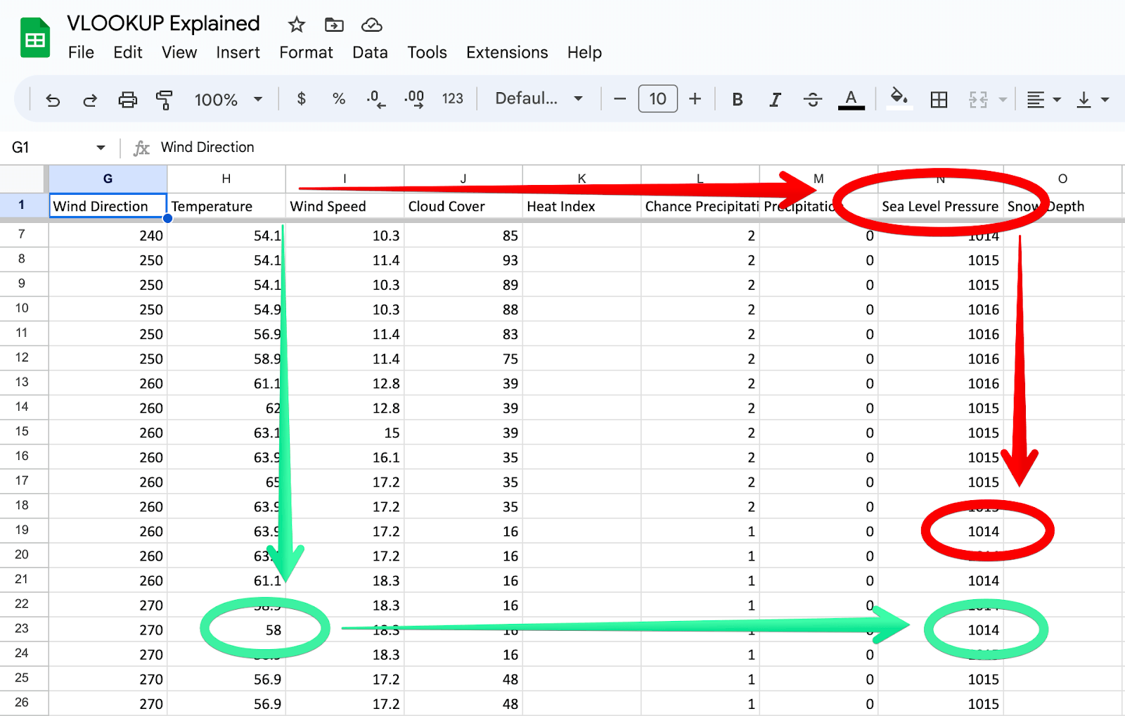
If your row is much longer, like we have in the weather data set imported from a CSV file, you should use the COLUMN function in the column-index parameter.

=ARRAYFORMULA(VLOOKUP(search-key, range, COLUMN(data-range), [sorted/not-sorted])

Note: specify the data range within the COLUMN function excluding the last column with data. For example, your data range is A2:D. Your VLOOKUP function should contain COLUMN (A2:C), otherwise it will return an Error - VLOOKUP evaluates to an out of bounds range.

10. How to VLOOKUP to the left

The VLOOKUP function works in two directions:

1. From top to bottom
2. From left to right

If you need to look up a column to the left, there is a workaround:

=VLOOKUP(search-key, {lookup-column,range-without-lookup-column}, column-index, [sorted/not-sorted])

Here are some peculiarities to know:

• lookup-column – specify the column to look up.
• range-without-lookup-column – specify the data range excluding the column to look up. 
• column-index – the number of the looked up column of the range-without-lookup-column from which the matching value will be returned. The index of the first column of the range-without-lookup-column is always 2.

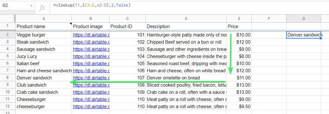
For example, we need to look up the Price column for the value “11” and learn the Product name that matches it. Here is how the formula will look:

=vlookup(11,{E2:E,A2:D},2,false)

11. VLOOKUP bottom to top in Google Sheets 

VLOOKUP usually searches from top to bottom, but what if we need to reverse this direction? 

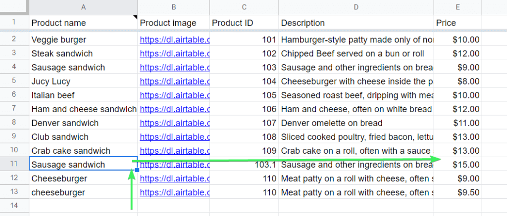
Let’s say, we have two items named ‘Sausage sandwich’ in our data set. They differ in price and we need to get it for the one which is closest to the bottom.

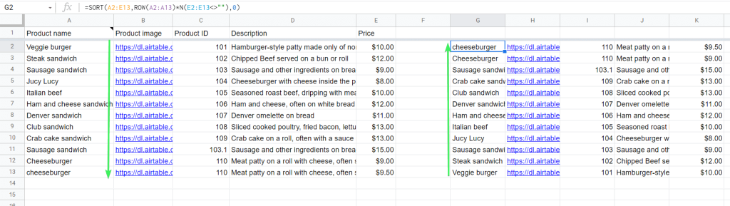
So, basically you need to flip your data range. You can do this with the following formula:

=SORT({data-range},ROW({first-column-in-range})*N({last-column-in-range}<>""),0)

In our case, this looks as follows:

=SORT(A2:E13,ROW(A2:A13)*N(E2:E13<>""),0)

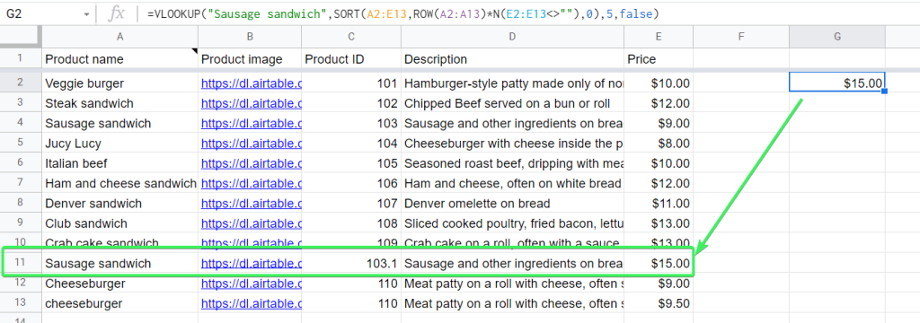
Now you can do the regular vlookup 🙂 However, the more advanced way is to best this formula into your VLOOKUP formula as follows:

=VLOOKUP(search-key,SORT({data-range},ROW({first-column-in-range})*N({last-column-in-range}<>""),0), column-index, [sorted/not-sorted]

In our example, here is how it looks

=VLOOKUP("Sausage sandwich",SORT(A2:E13,ROW(A2:A13)*N(E2:E13<>""),0),5,false)

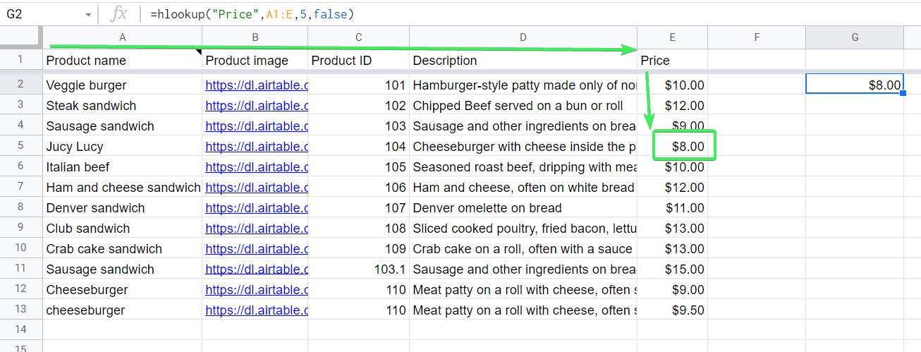
12. How to do a horizontal lookup: HLOOKUP function

HLOOKUP is VLOOKUP’s younger sister or brother. They even have similar formula syntax. The difference is that VLOOKUP searches first vertically and then horizontally; HLOOKUP searches first horizontally and then vertically. The function looks up the search-key in the first row of the data range, and then returns the value of the specified row.

HLOOKUP formula syntax:

=HLOOKUP(search-key, range, row-index, [sorted/not-sorted])

• range – specify the data range on any sheet to look up. HLOOKUP looks for the search key in the first row of the range.
• row-index – the number of the looked up row of the range from which the matching value will be returned. The index of the first row of the range is always 1.

This function works well with large-range data sets. For example, let’s look up the price of the item specified in the fifth row.

=hlookup("Price",A1:E,5,false)

13. How to VLOOKUP from another spreadsheet: VLOOKUP and IMPORTRANGE

VLOOKUP itself works within one Google Sheets document. If you need to look up a data set in another spreadsheet, nest VLOOKUP, and IMPORTRANGE. 

13.1 VLOOKUP IMPORTRANGE syntax

=VLOOKUP(search-key,IMPORTRANGE("spreadsheet-ID", "data_range"),column-index,[sorted/not-sorted])

Everything remains as is except for the range – you need to replace it with the IMPORTRANGE formula. Check out the VLOOKUP and IMPORTRANGE formula example, as well as other IMPORTRANGE capabilities in our blog post.

14. IF and VLOOKUP 

To customize your VLOOKUP formula result, you can nest VLOOKUP and IF differently. For example, here is the formula we used in the blog post “Trello Custom Fields to Google Sheets“:

={"Custom Field type","Custom Field name";
  arrayformula(
    if(len('All custom fields by cards'!E2:E)=0,,
      vlookup(
         'All custom fields by cards'!E2:E,
         {'All custom fields'!A2:A, 'All custom fields'!H2:H, 'All custom fields'!F2:F},
         {2,3},false
      )
    )
  )
}

The combination of ARRAYFORMULA, IF, and VLOOKUP allowed us to map Custom Field types by cards.

IF, LEN in the formula is a hack that allows you to switch off ARRAYFORMULA+VLOOKUP for empty cells. Without this hack, the formula would have worked with every row and returned #N/A for empty cells.

And here is how you can nest IF logic inside the VLOOKUP formula. Let’s say we have two data sets:

1. Products and their prices now
2. Products and their prices in 2019

We need to look up the price of "Italian Beef" depending on the year specified in the B1 cell. So, here is the VLOOKUP+IF formula:

=vlookup(
   "italian beef",
   if(B1=2019, 'Products 2019'!A2:E11, Products!A2:E11),
   5,
   false
)

The idea is that if B1 cell contains 2019, the VLOOKUP formula will return the price of Italian Beef in 2019. Otherwise, it will return the current price of the product.

Read more about Google Sheets logical expressions IF, IFS, AND, OR.

Is there any alternative to VLOOKUP in Google Sheets?   

The combination of INDEX and MATCH is considered a better alternative to VLOOKUP in Google Sheets, as well VLOOKUP Excel. Those are Google Sheets lookup functions, i.e. they return the value based on a search key or offset number:

• INDEX returns the cell value based on a specified row and column

INDEX(range, row-offset, column-index)

• MATCH returns the position of a search key in a specified range (either a single column or a single row)

MATCH(search-key, range, [search-type])

To use the combination of INDEX and MATCH instead of VLOOKUP, you need to replace either row-offset or column-index, or both with the MATCH formula. It may look as follows:

INDEX(range, MATCH(search-key, range, [search-type]), column-index)

Or 

INDEX(range, row-offset, MATCH(search-key, range, [search-type]))

Or

INDEX(range, MATCH(search-key, range, [search-type]), MATCH(search-key, range, [search-type]))

If you need to export data from somewhere into a spreadsheet, check out ready-to-use Google Sheets integrations and Excel integrations provided by Coupler.io. For now, Vlookup safely and streamline your data-centered activities. Good luck!

Back to Blog