Every Google Sheets user knows what the COUNT function is for. It returns the amount of numeric values in a data range. For counting not only numbers you can use COUNTA. And when your goal is to count data matching specific criteria, you should go with either COUNTIF or COUNTIFS. Read on to learn how they differ and what you can do with both functions in real-life cases.
Do you prefer watching to reading? Then check out this video about COUNT, COUNTIF, and COUNTIFS functions in Google Sheets by Railsware.
Google Sheets COUNTIF function to count values by one criterion
The COUNTIF function is a hybrid of COUNT and IF functions. It allows you to perform data counts based on a specific criterion.
COUNTIF Google Sheets syntax
=COUNTIF(data_range, "criterion")
data_range– Insert the range of cells to count.criterion– Insert the criterion (either number or string) to check thedata_rangeagainst. Alternatively, you can reference a cell that contains a criterion (in this case, don’t use quotation marks).
What you can count using COUNTIF in Google Sheets
With the COUNTIF function in Google Sheets you can count:
- Textual and numeric values by exact match
- Textual values by partial match
- Numeric values by a logical expression criterion
- The number of blank or non-blank cells
Let’s check out some formula examples for these cases below. For this, we’ve imported a data set from Airtable to Google Sheets using Coupler.io.

Coupler.io is a data integration solution to automate exports of data from multiple accounting, CRM, and other apps to Google Sheets, Excel, or BigQuery. Sign up to Coupler.io and schedule your data flow without coding at a custom frequency like every day except for Thursdays, every hour on Tuesdays, etc.
All the formula examples below are available in this spreadsheet.
Count textual and numeric values by exact match in Google Sheets
You can count the number of cells in the data range that contain a specific text or number.
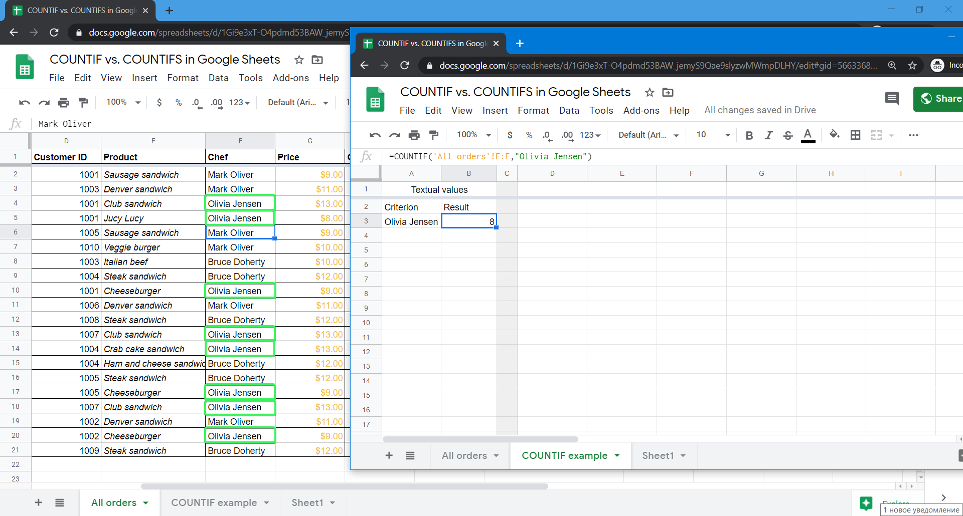
Google Sheets COUNTIF formula example for textual values
=COUNTIF('All orders'!F:F,"Olivia Jensen")
Interpretation:
Count all the Olivia Jensen values (criterion) in the F column of the All orders sheet (data_range).
Count textual values by partial match in Google Sheets
You can count the number of cells in the data range that contain a specific part of the text. For this, you’ll need to use wildcard characters: * or ?.
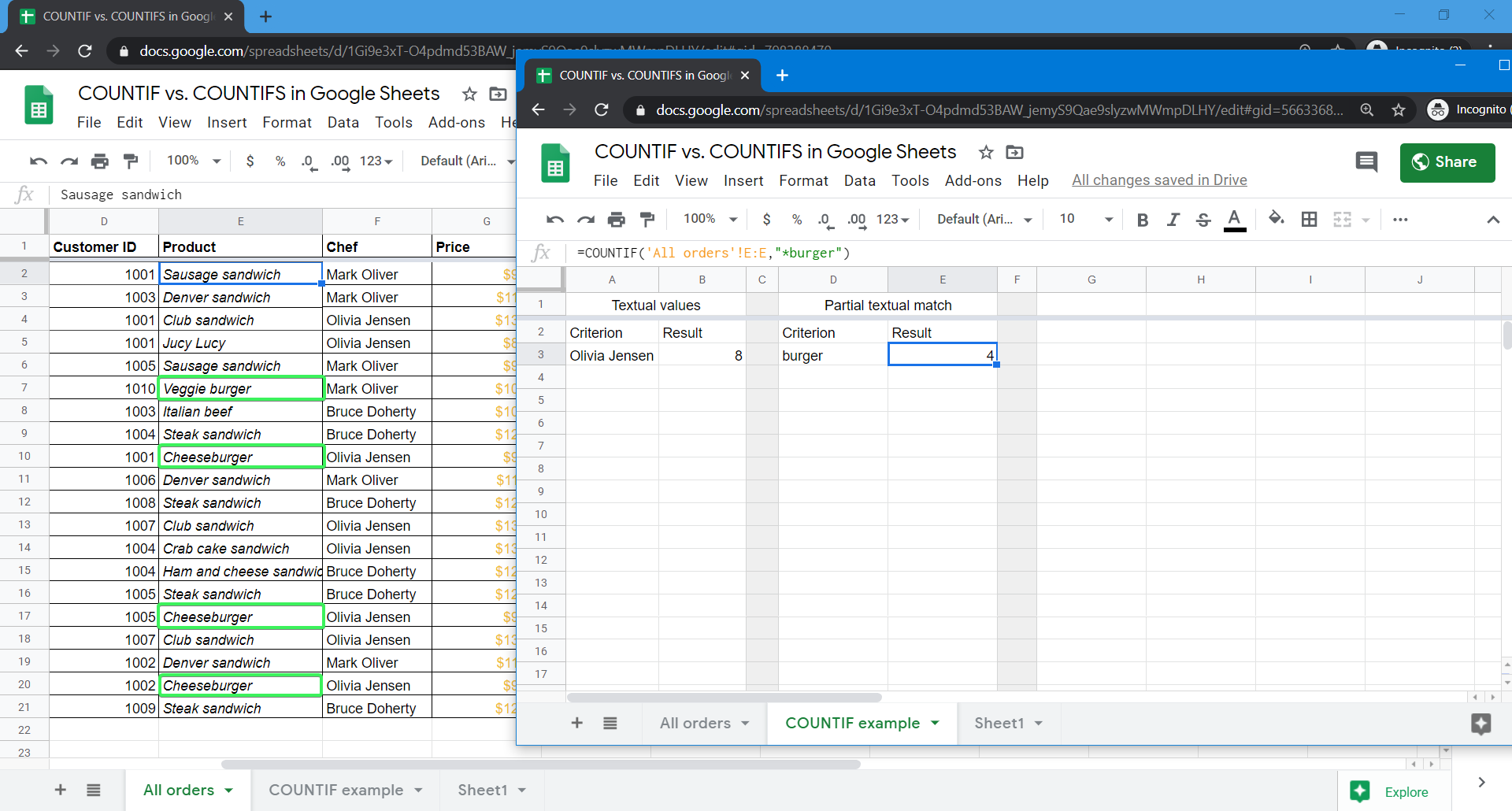
Google Sheets COUNTIF formula example for partial textual match
=COUNTIF('All orders'!E:E,"*burger")
Interpretation:
Count all the values that contain the word “burger” (criterion) in the E column of the All orders sheet (data_range).
Count numeric values in Google Sheets by a logical expression criterion: greater, less, or equal
You can count the number of cells in the data range that contain a numeric value that is less than, greater than, or equal to a specified number. These logical criteria can be combined with each other.
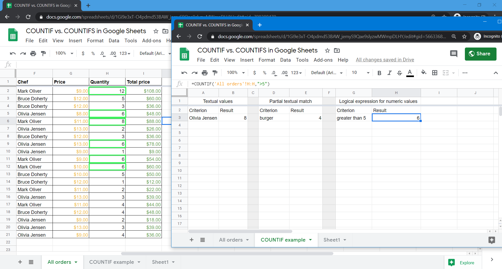
Google Sheets COUNTIF formula example for numeric values
=COUNTIF('All orders'!H:H,">5")
Interpretation:
Count all the values greater than 5 (criterion) in the H column of the All orders sheet (data_range).
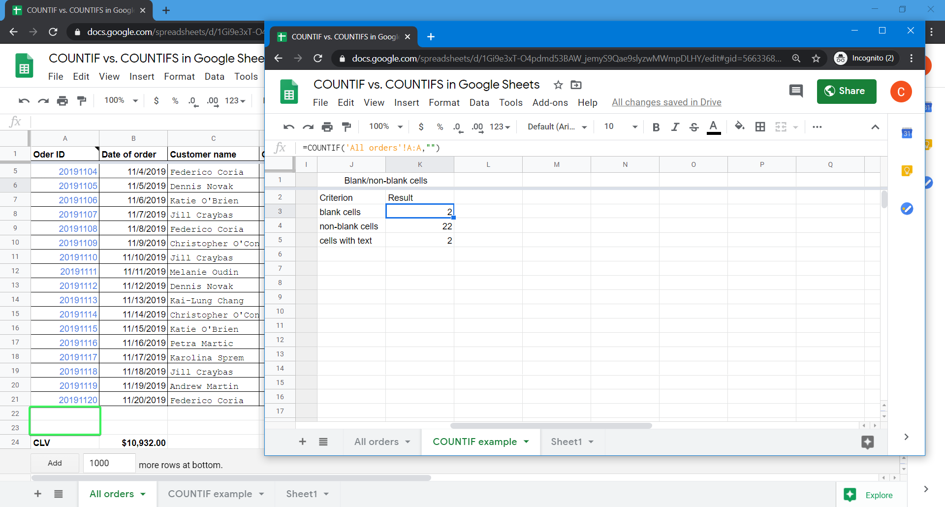
Google Sheets count blank and non-blank cells
You can count the number of blank or non-blank cells in the data range.
COUNTIF Google Sheets formula example to count blank cells
=COUNTIF('All orders'!A:A,"")
Google Sheets COUNTIF formula example to count non-blank cells with any value
=COUNTIF('All orders'!A:A,"<>")
The syntax is the same as for Excel COUNTIF not blank.
COUNTIF formula example in Google Sheets to count non-blank cells with a textual value
=COUNTIF('All orders'!A:A,"*")
Can I count values by multiple criteria with COUNTIF Google Sheets?
In Excel, COUNTIF supports multiple criteria. In Google Sheets, the COUNTIF function accepts only one data range and one criterion. Some suggest the following trick to count values across multiple criteria with:
=COUNTIF(data_range, “criterion#1”)+COUNTIF(data_range#2, “criterion#2”)+COUNTIF(data_range#3, “criterion#3”)…
However, this will only return the sum of separate counts based on separate criteria, which is unlikely to be what you need.
Let’s not reinvent the wheel, since there is an out-of-the-box solution: COUNTIFS.
COUNTIFS function Google Sheets to count values by multiple criteria
The COUNTIFS function is a hybrid of COUNT and IFS functions. It allows you to check multiple ranges with multiple criteria. The formula returns the count based on the criteria met.
Google Sheets COUNTIFS syntax
=COUNTIFS(data_range#1, "criterion#1",data_range#2, "criterion#2",data_range#3, "criterion#3",...)
data_range#1– Insert the range of cells to count.criterion#1– Insert the criterion (either number or string) to check thedata_range#1against. Alternatively, you can reference a cell that contains a criterion (in this case, don’t use quotation marks).data_range#2, "criterion#2",...– Additional ranges and criteria to check. The number of rows and columns in additional ranges must be equal to those in thedata_range#1.
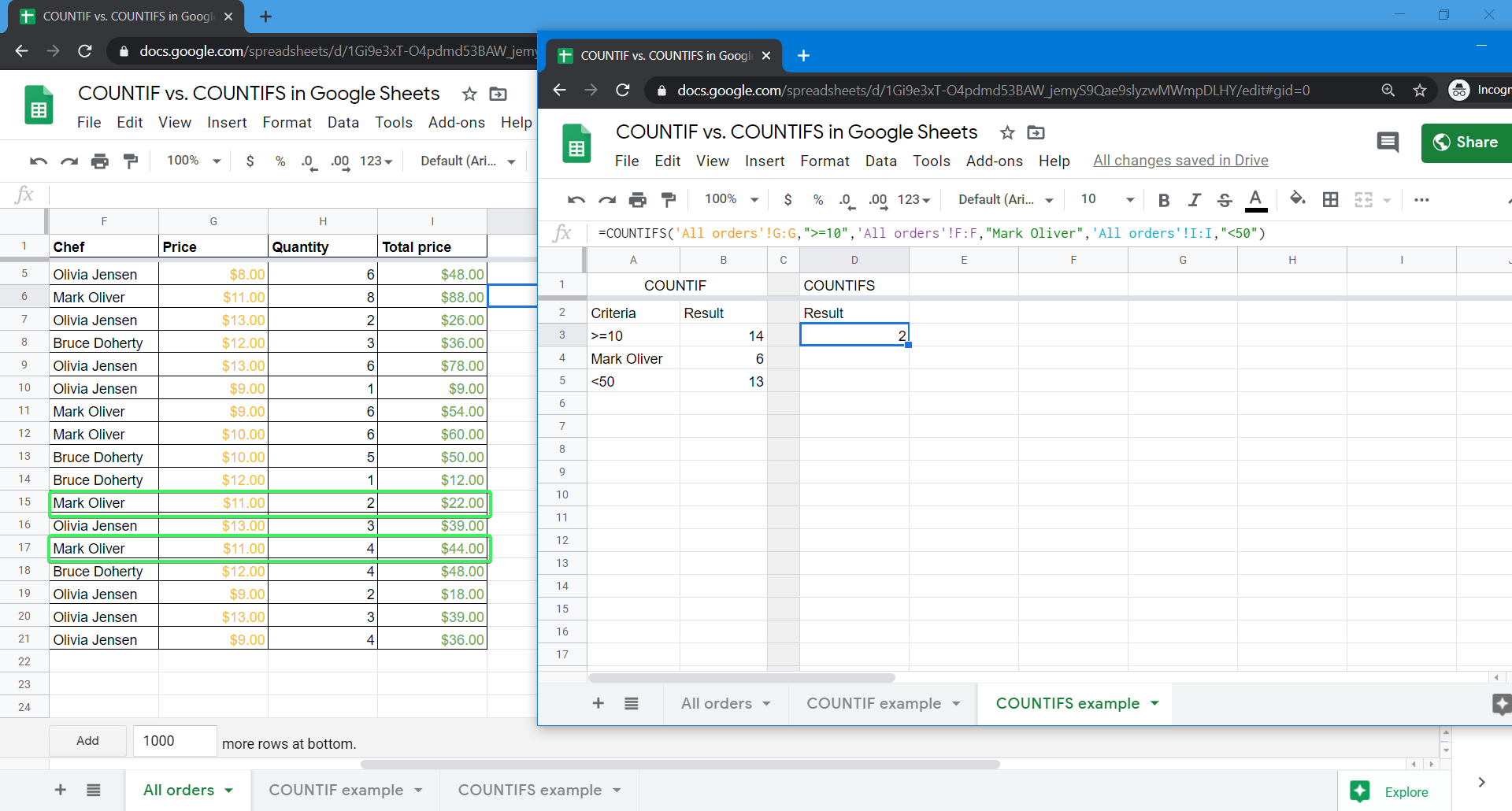
COUNTIFS Google Sheets formula example
=COUNTIFS('All orders'!G:G,">=10",'All orders'!F:F,"Mark Oliver",'All orders'!I:I,"<50")
Interpretation:
Count the values that meet all the following criteria:
1. Values in the G column of the All orders sheet (data_range#1) that are greater or equal to 10 (criterion#1).
2. Values in the F column of the All orders sheet (data_range#2) that contain “Mark Oliver” text exactly (criterion#2).
3. Values in the I column of the All orders sheet (data_range#3) that are less than 50 (criterion#3).
In this tab, you can check out the formula example and compare it to separate COUNTIF formulas based on the mentioned criteria.
How do you use Google Sheets COUNTIFS for the same range?
To check multiple criteria in the same column range, you need to use ARRAYFORMULA + SUM + COUNTIFS and place your criteria in the curly braces
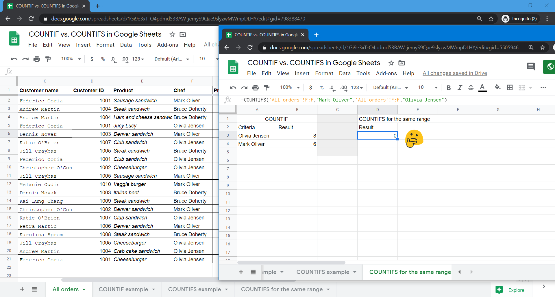
Let’s say you need to check multiple criteria in the same data range. For example, you want to count the values in the F column of the All orders sheet (data_range) that contain exact “Mark Oliver” (criterion#1) and the values that contain “Olivia Jensen” (criterion#2). You might have thought about the following:
=COUNTIFS(‘All orders’!F:F,”Mark Oliver”,’All orders’!F:F,”Olivia Jensen”)
Unfortunately, this won’t do because it acts like the AND function in Google Sheets: it’ll look for a value that is Mark Oliver and Olivia Jensen at the same time.
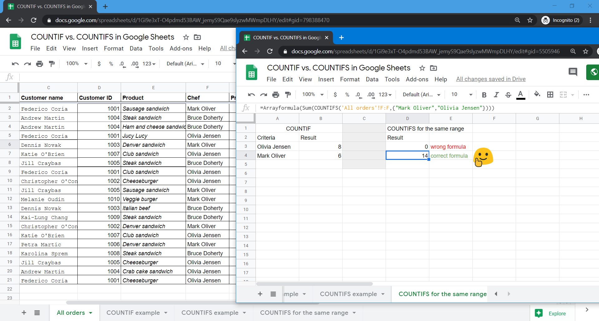
To check multiple criteria in the same column range, you need to use ARRAYFORMULA + SUM + COUNTIFS and place your criteria in the curly braces as follows:
=Arrayformula(
  Sum(
   COUNTIFS('All orders'!F:F,{"Mark Oliver","Olivia Jensen"})
  )
)
Use Google Sheets QUERY as a COUNTIFS alternative
Earlier we blogged about the Google Sheets QUERY function, which allows you to grab the data based on criteria and perform various data manipulations. You can use QUERY as an alternative to COUNTIFS:
- Use the
SELECTclause combined with theCOUNT()function to make a data count. - Use the
WHEREclause combined with theANDlogical function to set up multiple criteria.
Here is how the QUERY formula for counting values based on the multiple criteria will look:
| COUNTIFS formula | QUERY formula |
|---|---|
=COUNTIFS('All orders'!G:G,">=10",'All orders'!F:F,"Mark Oliver",'All orders'!I:I,"<50") | =QUERY('All orders'!F:I,"select count(F) where F='Mark Oliver' and G>=10 and I<50",0) |
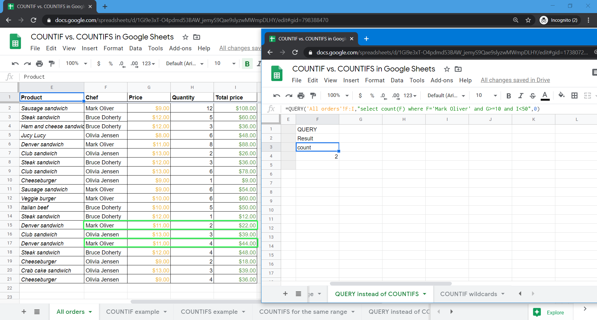
Check out the formula example in this tab. You may also be interested in how to use a combination of QUERY + IMPORTRANGE in Google Sheets.
How to count values by partial match check with COUNTIF & COUNTIFS wildcards Google Sheets
There are two wildcards you can use to check the partial match of the data range: ? and *.
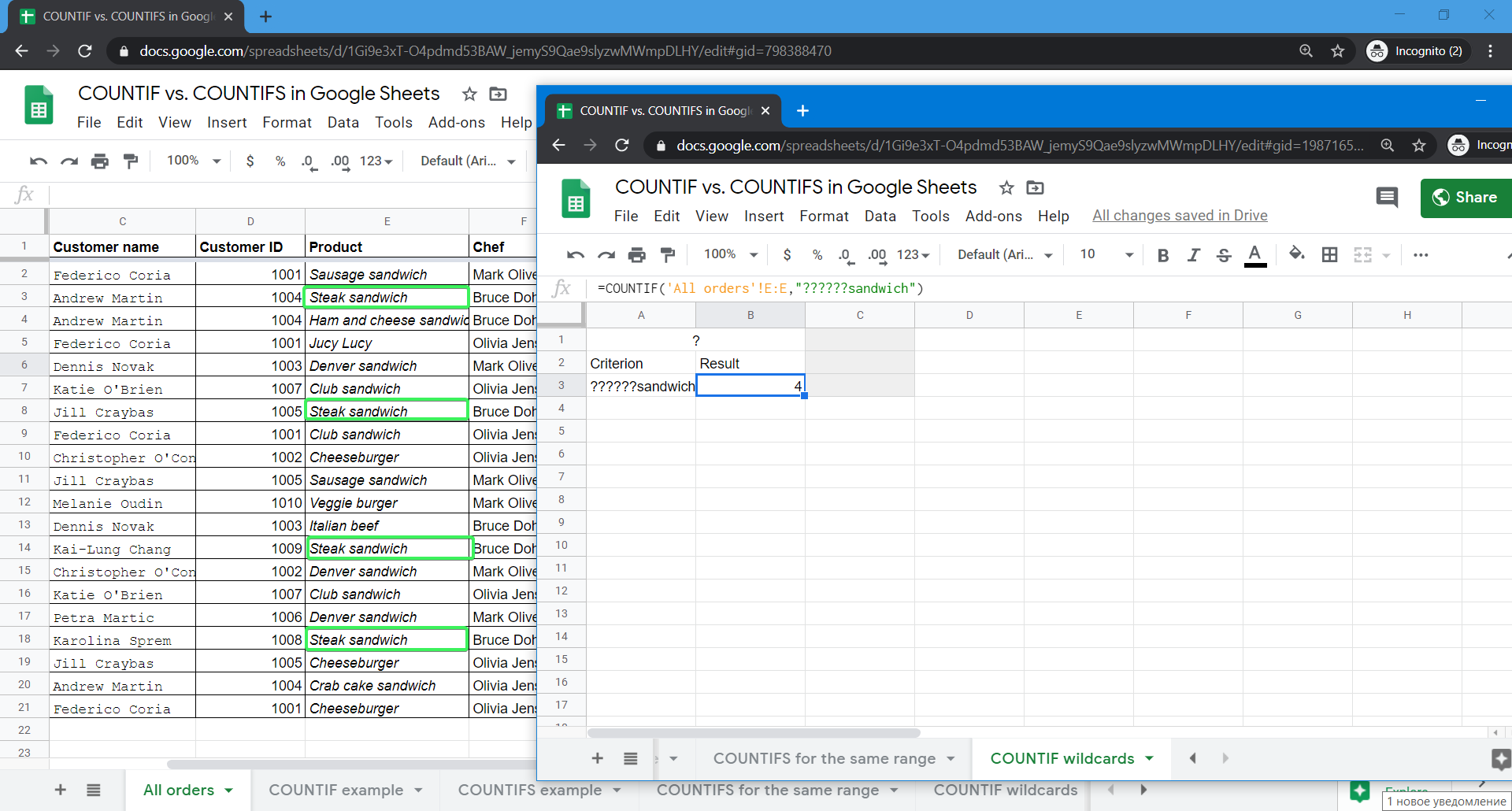
Google Sheets question mark wildcard (?)
The question mark (?) allows you to disguise one character you want to ignore. One question mark = one character. For example, "???ed" means that you’re looking for the 5-letter words that end with “ed“.
Google Sheets COUNTIF formula example with the question mark (?) wildcard
=COUNTIF('All orders'!E:E,"??????sandwich")
Interpretation:
Count the values in the E column of the All orders sheet (data_range) that contain the 14-letter wording that ends with “sandwich” (criterion).
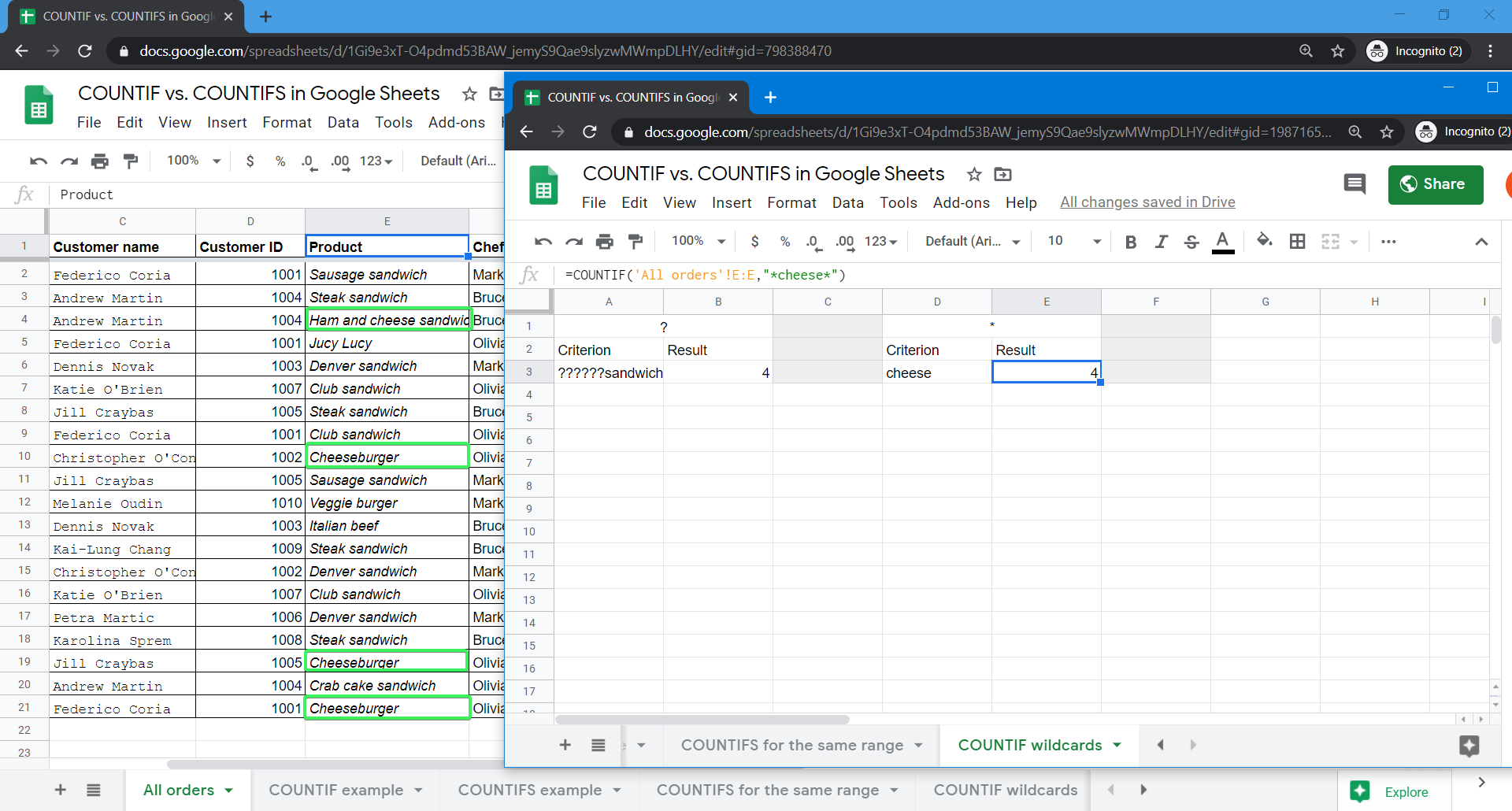
Google Sheets asterisk wildcard (*)
The asterisk (*) allows you to disguise any number of characters you want to ignore. For example:
"*sandwich"means that you’re looking for wordings that end with “sandwich“."sandwich*"means that you’re looking for wordings that start with “sandwich“."*sandwich*"means that you’re looking for any wordings that contain “sandwich“.
Google Sheets COUNTIF formula example with the asterisk (*) wildcard
=COUNTIF('All orders'!E:E,"*cheese*")
Interpretation:
Count the values in the E column of the All orders sheet (data_range) that contain “cheese“ in the wording (criterion).
Both examples are available in this tab.
Note: Use tilde sign (
~) before an asterisk (*) or a question mark (?) to treat them as simple signs. For example,"~**"means that you’re looking for the values that start with an asterisk “*“.
Where in real life you may need Google Sheets COUNTIF or COUNTIFS
The examples above will unlikely be useful in real life. However, both COUNTIF and COUNTIFS can do the job when you need to build complex dashboards. Check out the following use case that will unfold the practical value of these functions.
Use case: A live sales dashboard integrated with Pipedrive
Idea:
Import the data from sales management software (we picked Pipedrive as an example) and build a sales dashboard stuffed with actionable metrics and data visualizations. Moreover, the dashboard will be updated automatically every day!
Step 1: Pipedrive data import
First we need to import our deals from Pipedrive to Google Sheets and automate data updates in the future. Coupler.io, the tool that we’ve already mentioned above, can handle these tasks easily. You’ll need to do the following:
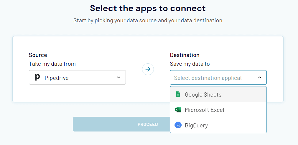
- Sign up to Coupler.io, click Add importer, and select Pipedrive as a source app and Google Sheets as a destination app.
- Configure what data you want to export from Pipedrive and where to load it in Google Sheets.
- Set up a schedule for automatic data refresh of your exported Pipedrive records.
Step 2: Building the sales dashboard
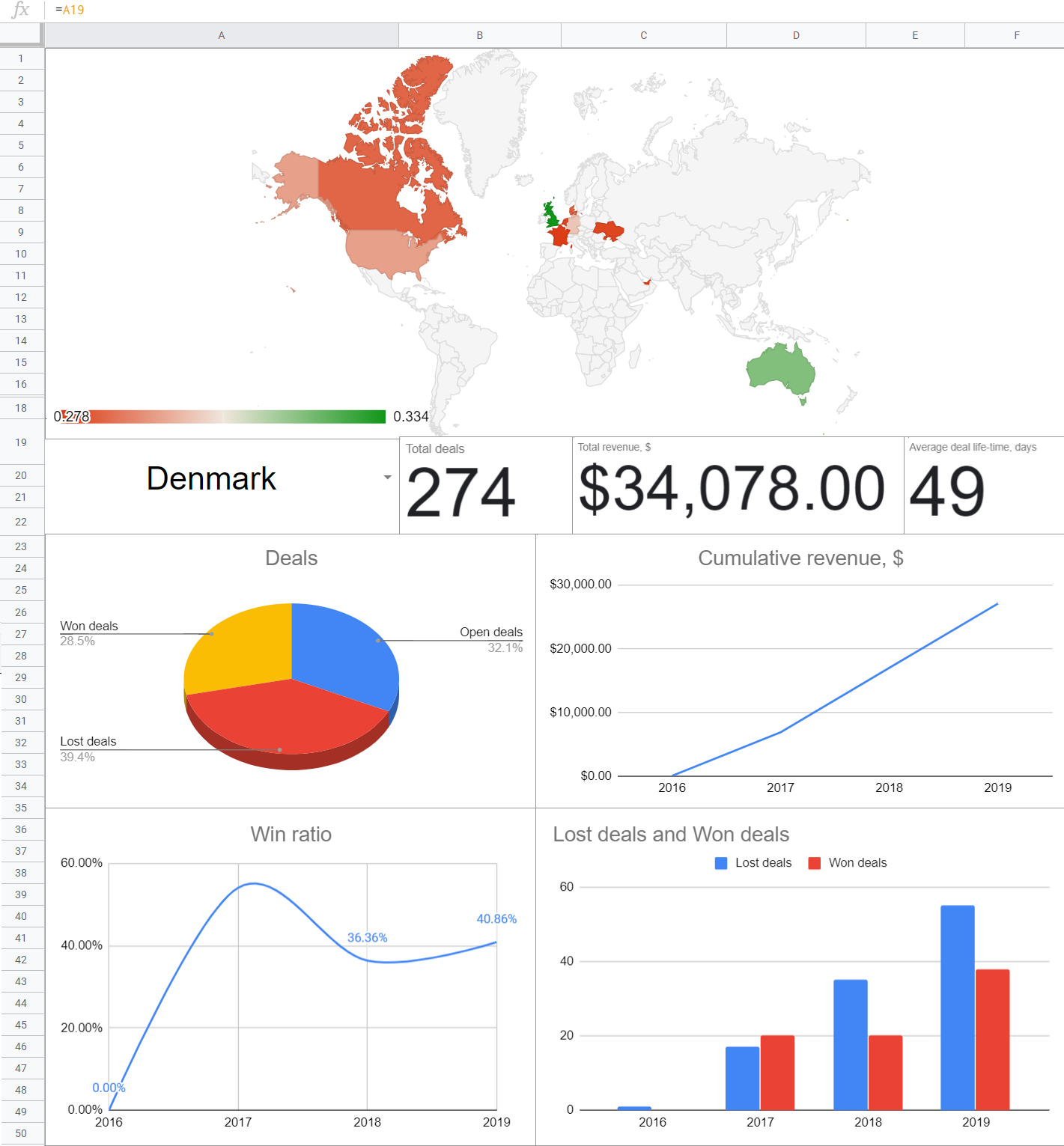
The sales dashboard template, which you can download and adjust for your project, displays multiple sales metrics. But in terms of the COUNTIF usage, we’ll need the following ones:
- Geo chart with a conversion rate
- Deals breakdown (won, open, and lost)
- Win rate
Geo chart with a conversion rate
Conversion rate shows the ratio of won deals to total deals. To count the total deals, we’ll need the COUNTA function, whereas COUNTIF will help us return the won deals. Apply the FILTER function to sort results by the country and here is the formula:
=COUNTIF(Filter(Deals!AL2:AL,Deals!Z2:Z=A61),"won")/
 COUNTA(Filter(Deals!AL2:AL,Deals!Z2:Z=A61))
Deals!AL2:AL– the status column of the imported dataDeals!Z2:Z– the org_id.address column of the imported dataA61– a cell with the country name
Deals breakdown (won, open, and lost)
A similar formula will return the number of deals by status. Here is how it looks for the lost deals:
=IF(
  ISBLANK(A19),
  COUNTIF(Deals!AL2:AL,"lost"),
  COUNTIF(Filter(Deals!AL2:AL,Deals!Z2:Z=A19),"lost")
)
Deals!AL2:AL– the status column of the imported dataDeals!Z2:Z– the org_id.address column of the imported dataA19– a cell with the country name
Win rate
Win rate is the ratio of won deals to closed deals, which in turn equals the sum of lost deals and won deals. COUNTIF will help us handle this complex calculation:
=IF(
  ISBLANK(A19),
  IFERROR(
   COUNTIF(
    Filter(Deals!AL2:AL,Deals!CN2:CN=2016),"won")/
   (COUNTIF(
     Filter(Deals!AL2:AL,Deals!CN2:CN=2016),"won")+
    COUNTIF(
     Filter(Deals!AL2:AL,Deals!CN2:CN=2016),"lost")),
   "No closed deals"),
  IFERROR(
   COUNTIF(
    Filter(Deals!AL2:AL,Deals!Z2:Z=A19,Deals!CN2:CN=2016),"won")/
   (COUNTIF(
    Filter(Deals!AL2:AL,Deals!Z2:Z=A19,Deals!CN2:CN=2016),"won")+
   COUNTIF(
    Filter(Deals!AL2:AL,Deals!Z2:Z=A19,Deals!CN2:CN=2016),"lost")),
   "No closed deals")
)
Deals!CN2:CN– the Year columnDeals!AL2:AL– the status column of the imported dataDeals!Z2:Z– the org_id.address column of the imported data
For more about this interactive dashboard, read our blog post How to Build Sales Tracker with Google Sheets.
Use COUNTIF or COUNTIFS for your projects
Now you know how to count with COUNTIF/COUNTIFS. Will this knowledge be helpful? We hope so and encourage you to check other Google Sheets functions we’ve described in the Coupler.io blog. The more you know, the better your reporting and dashboards will work. Good luck with your data!