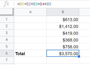
The most primitive way to total cells in Google Sheets is to add the cell references to the formula and put plus (+) signs between them. For example:
=B1+B2+B3+B4+B5
For longer ranges of cells, such as an entire column or row, this solution is not handy at all. Instead, you should use the SUM function or one of its derivatives: SUMIF and SUMIFS. Let’s check out how the native functions work and which use cases are a fit for them. Or you can check out our short video about how to total a column in Google Sheets using these functions.
Google Sheets SUM to total values
SUM is a Google Sheets function to return a total of numbers or cells, or both specified numbers and cells. The SUM syntax has several variations depending on what you’re going to total.
Google Sheets SUM syntax to total values
=SUM(value1,value2,value3,…)valueis a numeric value
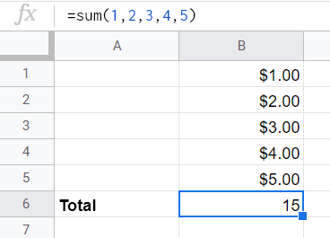
Google Sheets SUM basic formula example
=sum(1,2,3,4,5)
Google Sheets SUM to total a cell range
Google Sheets SUM syntax to total cells
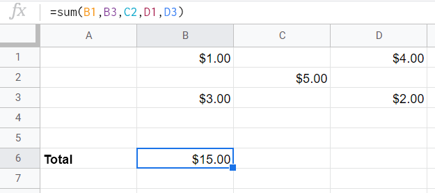
=SUM(cell-range)cell-rangeis the range of cells to total. The range can be specified using commas for scattered cells likeA1,B2,C3, or a colon for integral cell ranges likeA1:A100.
Google Sheets SUM formula example for scattered cells
=sum(B1,B3,C2,D1,D3)
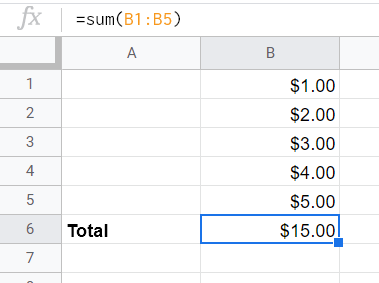
Google Sheets SUM formula example for an integral cell range
=sum(B1:B5)
Google Sheets SUM to total values and cells
Google Sheets SUM function syntax to total values and cells
=SUM (value1, value2,...,cell-range)Google Sheets SUM formula example to total values and cells
=sum(1,2,B3,B4:B5)

How to SUM a column in Google Sheets
Now you know the syntax of the SUM formulas, so let’s check out how they work on real-life data. We’ve imported some records from HubSpot to Google Sheets using Coupler.io, a no-code reporting automation solution.
So, with the data imported to Google Sheets, we can proceed to SUM formula examples.
SUM a limited range from a column in Google Sheets
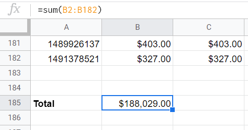
If you need to return the total of a limited range from a column, e.g. B2:B182, a simple SUM syntax will do:
=sum(B2:B182)
If you want to return the total in the bottom of your column range, type the equal sign (=), and Google Sheets will suggest you the SUM formula itself.
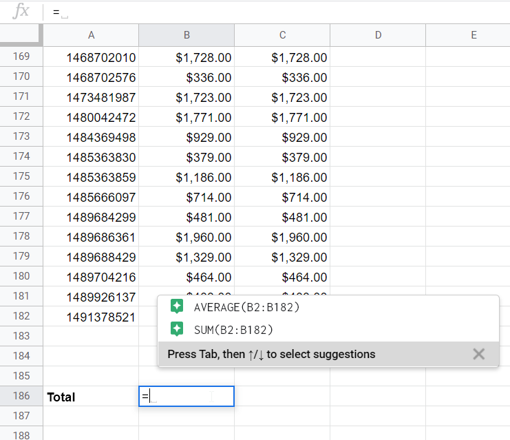
Note: This hack works only within 5 rows below the last value in a column.
SUM an entire column in Google Sheets
If you need to total an entire column, specify the column range as follows:
=sum(B2:B)
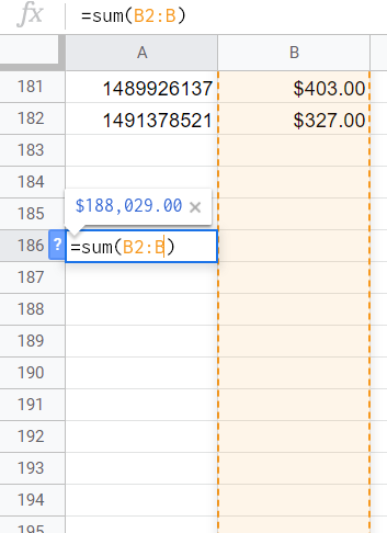
Now, every new value within the column will be added to the total value, so you won’t have to manually tweak the SUM formula.
How to SUM a row in Google Sheets
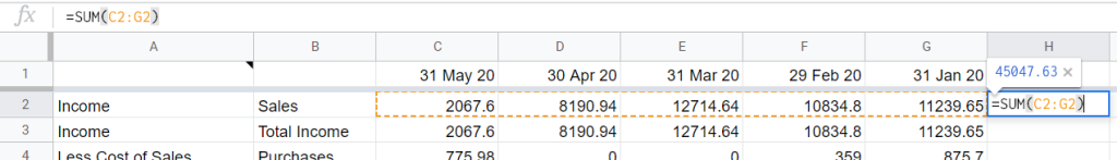
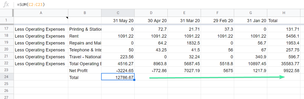
For this use case, we took a Profit and Loss report that we imported using the Xero Reports to Google Sheets integration. Now, let’s use SUM to total values from row 2.
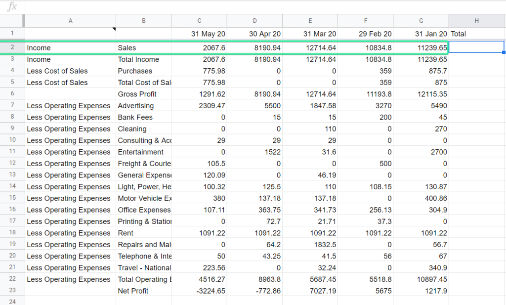
Here is the SUM formula to total the row values:
=SUM(C2:G2)
How to return SUM of multiple rows in one column in Google Sheets
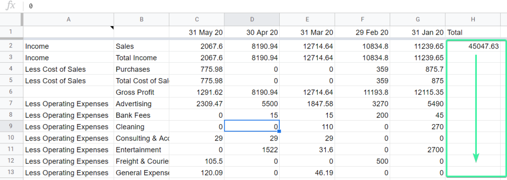
The SUM formula above worked well, but is it possible to expand it to other rows using ARRAYFORMULA?
Unfortunately, SUM + ARRAYFORMULA doesn’t expand: =ARRAYFORMULA(SUM(C2:G2)) will give a single number.
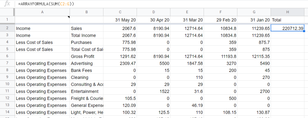
But there is a workaround..even three.
Workaround#1: Sum multiple rows in Google Sheets using Coupler.io
Coupler.io is a reporting automation solution to import data to Google Sheets from cloud services. In addition to automating dataflow, Coupler.io lets you organize your data before it hits the spreadsheet.
You only need to select your source app in the form below and click Proceed to get started. Create a Coupler.io account for free and connect your data source, be it a spreadsheet, database, accounting app, etc.
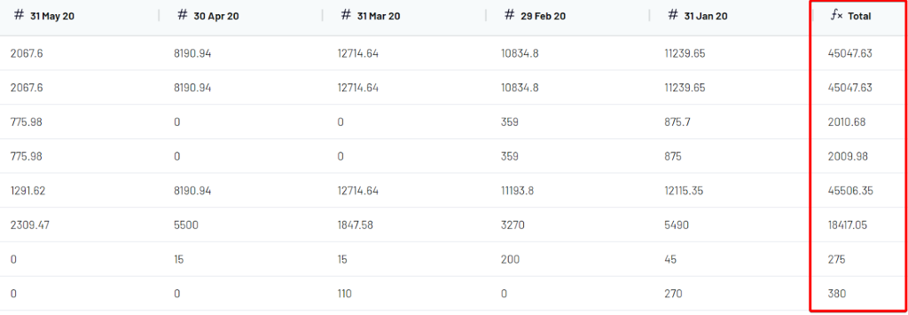
Once you select the data to import to Google Sheets, you’ll be able to organize it using filters and data transformation options. Click Formula, add a name for the new column (e.g., Total), and enter the needed columns to sum:
{31 May 20}+{30 Apr 20}+{31 Mar 20}+{29 Feb 20}+{31 Jan 20}
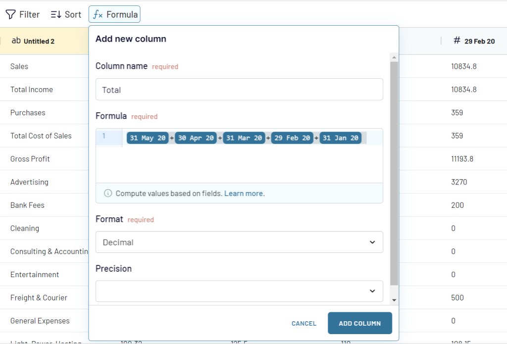
Click Add column and there you go!
Now you can proceed with the setup to load your data to the needed spreadsheet.
This way you can sum columns from one or multiple sources. Since Coupler.io supports Google Sheets both as a source and destination, you can use it as a better alternative to IMPORTRANGE or even QUERY+IMPORTRANGE.

Import your data to Google Sheets and transform it on the go with Coupler.io
Get started for freeWorkaround#2: Sum multiple rows with ARRAYFORMULA in Google Sheets
With this workaround, you don’t need the SUM function at all. The idea is to manually add the columns and use ARRAYFORMULA to expand the results. Here is the formula for our case:
=arrayformula(if(len(C2:C)=0,,(C2:C+D2:D+E2:E+F2:F+G2:G)))
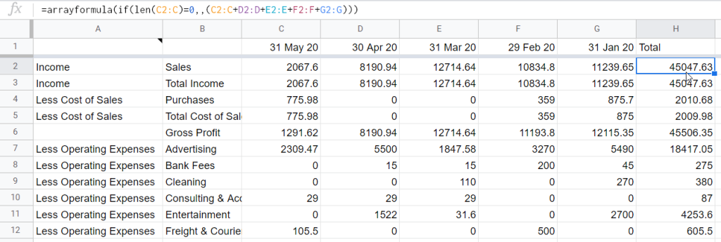
Note:
if(len(C2:C)=0is needed to remove “0” for empty rows.
Read our Guide of Using ARRAYFORMULA in Google Sheets.
Workaround#3: Sum multiple rows with ARRAYFORMULA, MMULT, TRANSPOSE, and COLUMN in Google Sheets
For this workaround, we’ll need to nest four functions: ARRAYFORMULA, MMULT, TRANSPOSE, and COLUMN. Here is how the formula looks:
=ARRAYFORMULA(MMULT(C2:G23,TRANSPOSE(COLUMN(C2:G23)^0)))
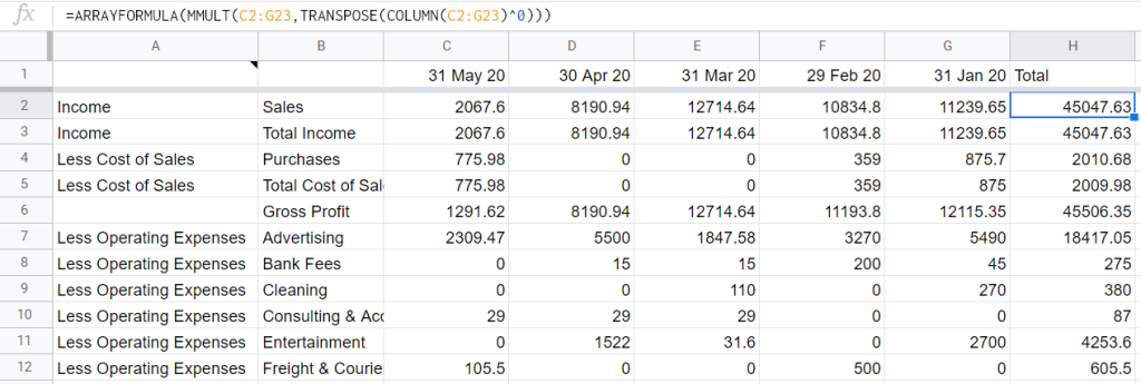
MMULT is an array function to multiply matrices. Our first matrix is C2:G23. The second matrix must have the number of rows equal to the number of columns in the first matrix – five, in our case. This is how it should look:
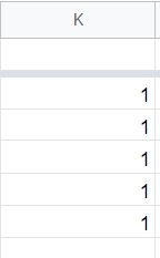
Instead of manually tailoring the matrix we need, we’ll use the combination of two functions, TRANSPOSE and COLUMN, in the following way: TRANSPOSE(COLUMN(C2:G23)^0)
In the end, wrap up everything with ARRAYFORMULA.
The drawback of this workaround is that you have to specify the exact range of columns.
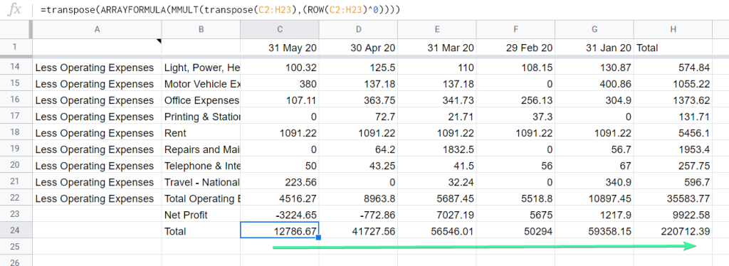
How to return SUM of multiple columns in one row in Google Sheets
Since we got the total column, let’s get the total row beneath the data set as well. MMULT nested with ARRAYFORMULA, TRANSPOSE, and ROW will help with that. Here is how it looks:
=TRANSPOSE(ARRAYFORMULA(MMULT(TRANSPOSE(C2:H23),(ROW(C2:H23)^0))))
Let’s wrap up with SUM for now, since we have more interesting cases with SUMIF and SUMIFS.
Google Sheets SUMIF to sum a data range on a condition
SUMIF is a Google Sheets function to return a total of cells that match a single specific criterion. Put simply, the SUMIF function filters the range according to the specified criteria and sums values based on this filter. The syntax is the same as SUMIF Excel.
Google Sheets SUMIF syntax
=SUMIF(criterion-range,"criterion",range-to-sum)criterionis a condition to filter data.criterioncan be a number, a text string, a cell reference, as well as a variety of conditions, such as greater than or equal to.criterion-rangeis a data range to examine based on thecriterionrange-to-sumis a data range with values to total. This parameter is optional and can be omitted in cases whencriterion-rangeis the range with values to total.
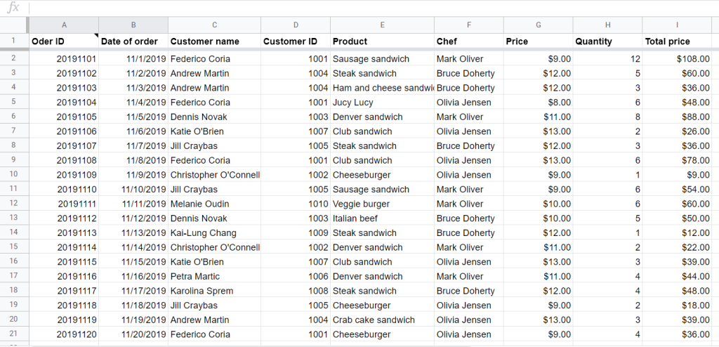
Now, let’s check out SUMIF formula examples with different criteria cases. For this, we’ll use a dummy data range that was already featured in the blog post COUNTIF vs. COUNTIFS. It’s an extract of a sandwich store’s database, in which you can see Product, Price, Quantity, and other columns. By the way, this data set was imported from Airtable to Google Sheets.
Google Sheets SUMIF by a logical expression criterion: greater, less, or equal
Use one of the following logical operators to build a criterion for the SUMIF formula:
| Logical expression | Logical operator |
| greater than | > |
| less than | < |
| equal to | = |
| greater than or equal to | >= |
| less than or equal to | <= |
| except for | <> |
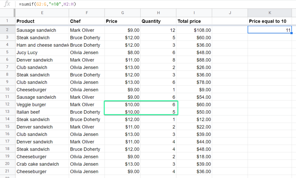
For example, let’s total the amount of products with the price equal to 10.
=sumif(G2:G,"=10",H2:H)
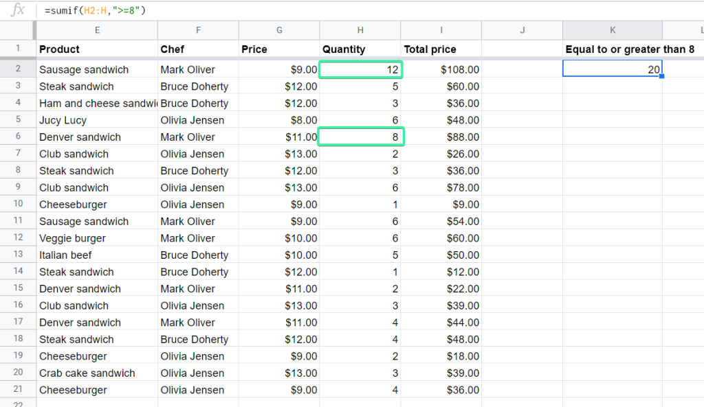
Another formula example is to total the amount of products that are greater than or equal to 8. Bring to notice that this formula syntax is free of range-to-sum, since the function will total the values from criterion-range:
=sumif(H2:H,">=8")
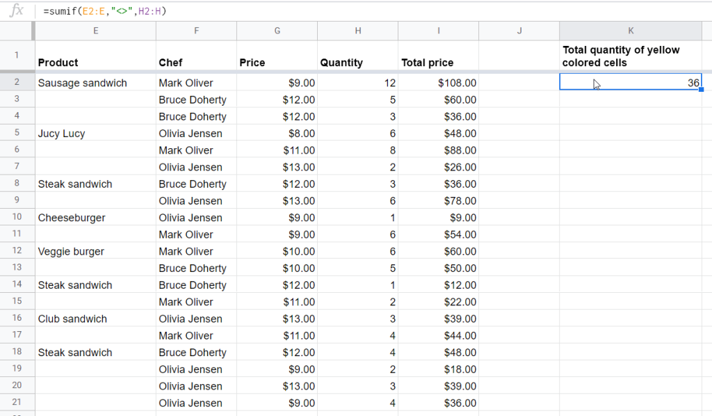
Google Sheets SUMIF: how to sum the not empty cells
The use of the logical operator “except for” (<>) without any text string or cell reference means that the criterion is “not empty cells“. For example,
=sumif(E2:E,"<>",H2:H)
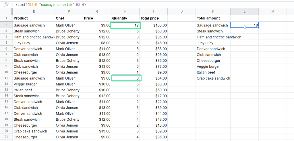
Google Sheets SUMIF: how to sum cells by exact match
The exact match criterion can be specified as a text string, numeric value, or a cell reference. For example, here is the SUMIF formula to total the amount of a Sausage sandwich:
=sumif(E2:E,"sausage sandwich",H2:H)
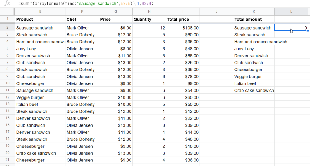
Google Sheets SUMIF: how to sum by a case-sensitive criterion
SUMIF does differentiate between upper- and lower-case letters. That’s why in the formula example above, SUMIF totaled the amount of Sausage sandwich, though we specified "sausage sandwich" as the criterion. If case sensitivity matters, you can use the following workaround:
=SUMIF(ARRAYFORMULA(FIND("criterion",criterion-range)),1, range-to-sum)So, our formula will look like this and return “0” since there is no match to the criterion:
=sumif(arrayformula(find("sausage sandwich",E2:E)),1,H2:H)
How to expand SUMIF Google Sheets formula in a column: ARRAYFORMULA+SUMIF
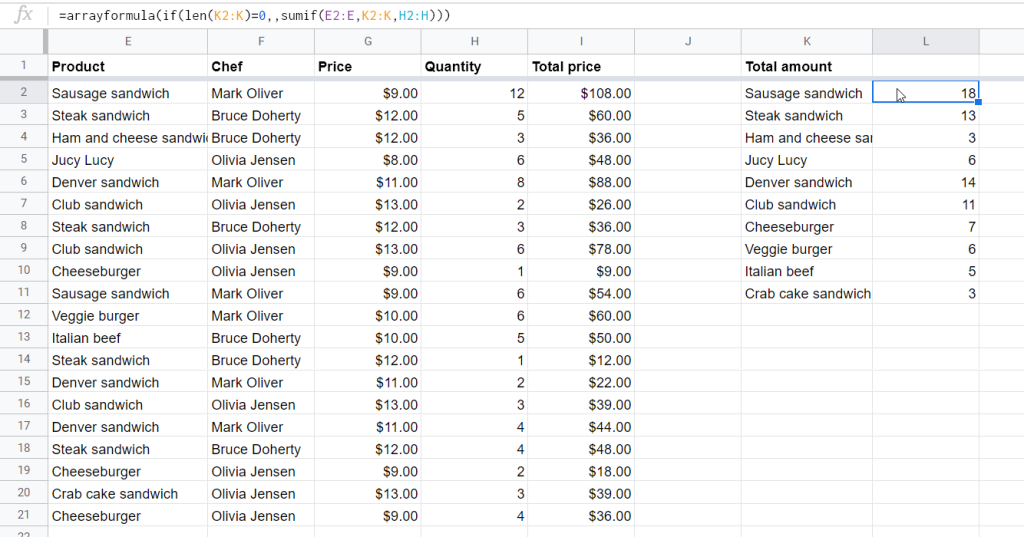
Let’s expand the SUMIF formula to calculate the total amount of other products.
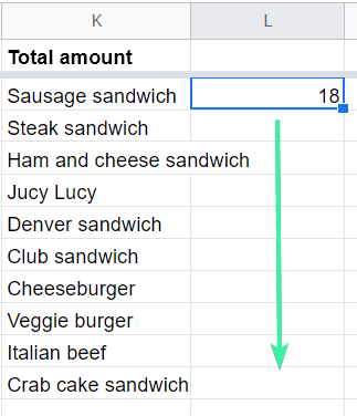
Here is the syntax you should use:
=ARRAYFORMULA(SUMIF(criterion-range,criteria,range-to-sum)In our case, the SUMIF formula will look as follows:
=arrayformula(if(len(K2:K)=0,,sumif(E2:E,K2:K,H2:H)))
Note:
if(len(K2:K)=0is needed to remove “0” for empty rows.
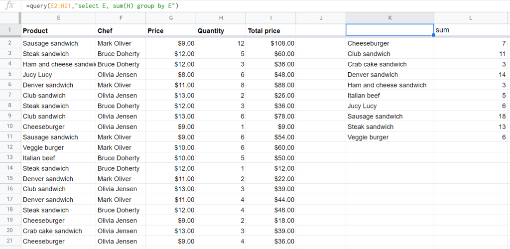
How to sum and group values by a certain condition in Google Sheets: QUERY+SUM
Here is an alternative solution to the SUMIF formula above. The idea is to extract unique values from the Product column and return the total amount of each product with a single formula. The QUERY function can easily do that as follows:
=query(E2:H21,"select E, sum(H) group by E")
Read our blog post for more about using QUERY in Google Sheets.
Google Sheets SUMIF: how to sum by partial match
The partial match criterion is when you need to total cells in range-to-sum if the cells in criterion-range contain specific characters. To tailor a partial match criterion, you’ll need to use the following wildcards:
- Question mark (
?) to disguise every single character of a text string. For example,"????er"means that thecriterionis a 6-letter word that ends with"er". - Asterisk (
*) to disguise any number of characters of a text string. For example,"*er*"means that that thecriterionis any word that contains"er". - You can also concatenate wildcards and cell references. For example,
"+"&C5means that thecriterionis a text string that ends with the value from the C5 cell.
Let’s check out the common examples:
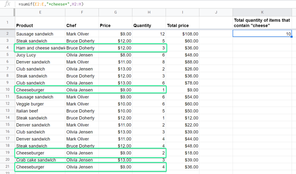
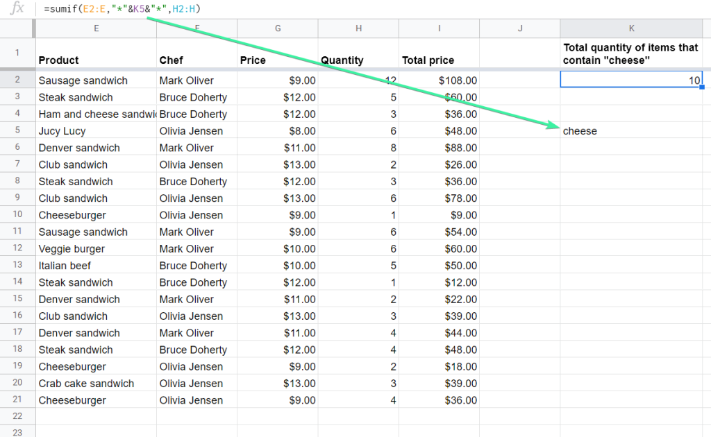
SUMIF formula to total all items that contain “cheese” in their naming:
=sumif(E2:E,"*cheese*",H2:H)
And here is what this SUMIF formula will look if we use a cell reference concatenated with wildcards:
=sumif(E2:E,"*"&K5&"*",H2:H)
How to sum cells by color with SUMIF in Google Sheets
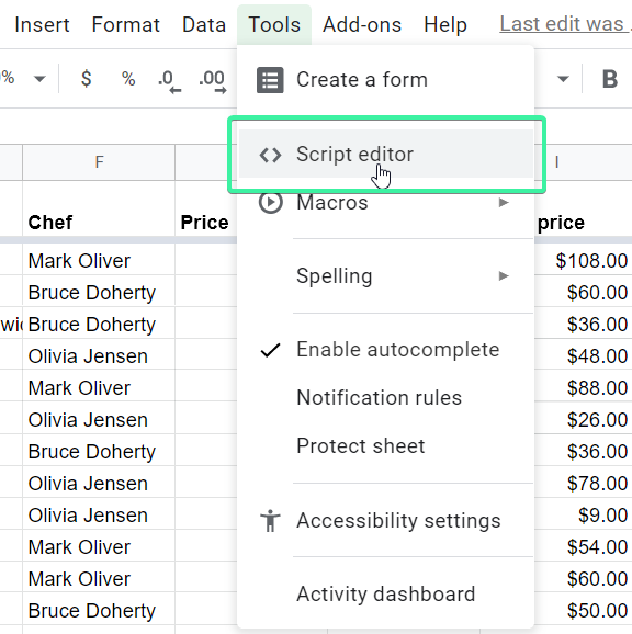
Google Sheets doesn’t have this feature built-in. However, you can do it yourself using the Script editor. It won’t take more than a minute.
- Open Script editor in your spreadsheet: go to Tools => Script editor
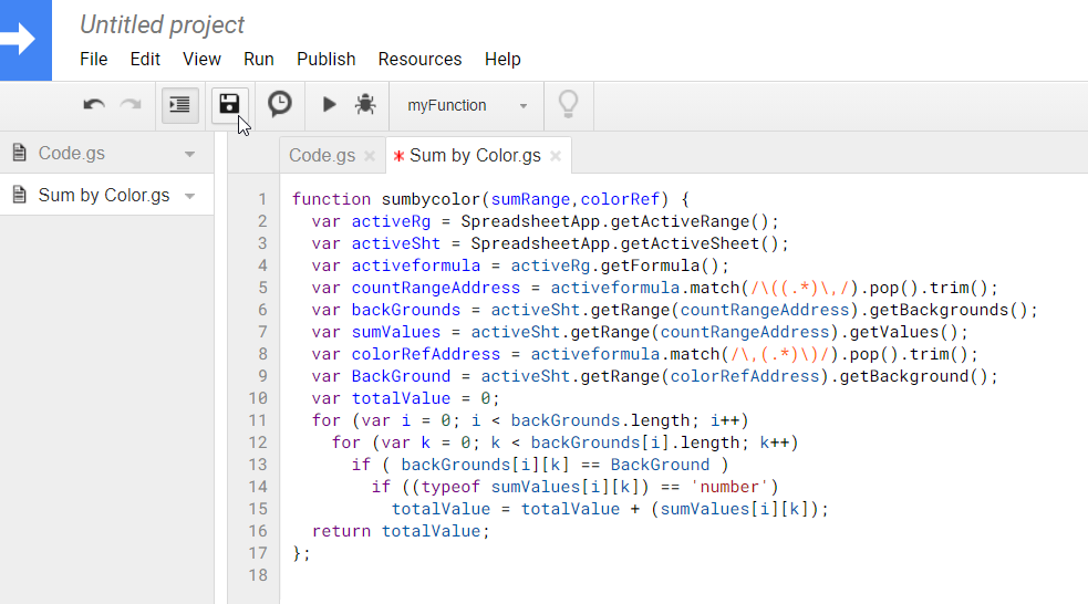
- Open a new script file: go to File => New => Script file. Name the file as you want.

- Copy and paste the following script to replace the original code.
function sumbycolor(sumRange,colorRef) {
  var activeRg = SpreadsheetApp.getActiveRange();
  var activeSht = SpreadsheetApp.getActiveSheet();
  var activeformula = activeRg.getFormula();
  var countRangeAddress = activeformula.match(/\((.*)\,/).pop().trim();
  var backGrounds = activeSht.getRange(countRangeAddress).getBackgrounds();
  var sumValues = activeSht.getRange(countRangeAddress).getValues();
  var colorRefAddress = activeformula.match(/\,(.*)\)/).pop().trim();
  var BackGround = activeSht.getRange(colorRefAddress).getBackground();
  var totalValue = 0;
  for (var i = 0; i < backGrounds.length; i++)
    for (var k = 0; k < backGrounds[i].length; k++)
      if ( backGrounds[i][k] == BackGround )
        if ((typeof sumValues[i][k]) == 'number')
          totalValue = totalValue + (sumValues[i][k]);
  return totalValue;
};
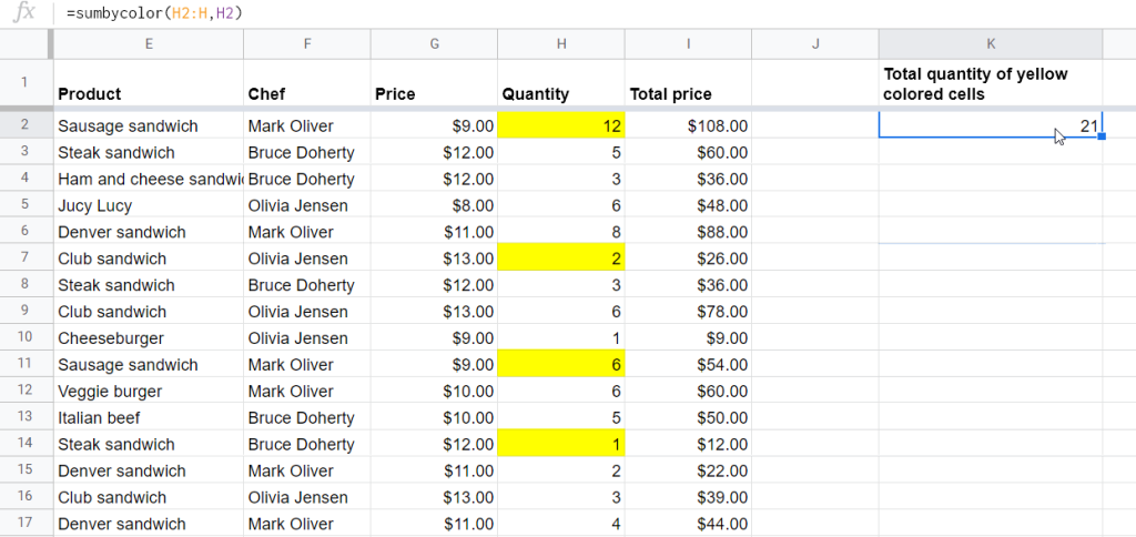
Click Save (you might be offered to give a name to your project) and get back to the Google Sheets doc.
Now, you have the SUMBYCOLOR function with the following syntax:
=SUMBYCOLOR(range-to-sum,colored-cell-criterion)range-to-sumis a data range with values to total, as well as to examine based on thecolored-cell-criterion.colored-cell-criterionis a colored cell that defines the background color to filter and sum the data.
Here is a formula example:
=sumbycolor(H2:H,H2)
Kudos to ExtendOffice for the workaround. Check out their blog post if you also want to count cells by color.
Import your data to Google Sheets and transform it on the go with Coupler.io
Get started for freeGoogle Sheets SUMIFS to sum a data range based on multiple criteria
SUMIFS is the youngest child in the SUM family. It lets you total values considering two or more criteria across different ranges.
Google Sheets SUMIFS syntax
=SUMIFS(range-to-sum,criterion-range1,"criterion1",criterion-range2,"criterion2",...)The parameters are the same as with SUMIF, but you can add multiple criteria to a single formula.
SUMIFS works by the AND logic: to get the total sum, all the specified criteria must be met, otherwise the formula will return “0”.
SUMIFS Google Sheets formula example
Let’s get back to our data set and total the amount of items by the following criteria:
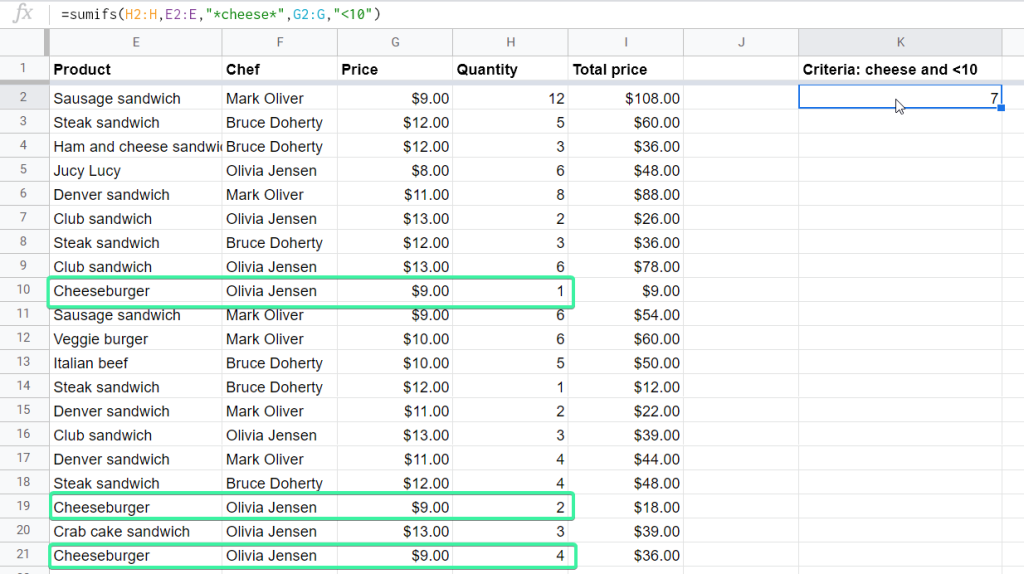
- Product name must contain “cheese“
- Product price must be less than $10
Here is the SUMIFS formula:
=sumifs(H2:H,E2:E,"*cheese*",G2:G,"<10")
How to expand SUMIFS formula in Google Sheets
SUMIF can be nested with ARRAYFORMULA to expand the results. With SUMIFS, you can’t do that. However, if you badly need to expand SUMIFS, check out the workaround formulas for this.
SUMIF a data range based on multiple criteria with OR logic in Google Sheets
SUMIFS returns a sum of values if all criteria are met based on the AND logic. The OR logic is when any of the specified criteria is met. This can be done with an advanced SUMIF formula.
SUMIF Google Sheets formula when any of the two criteria is met
=SUMIF(criterion-range,"criterion1",range-to-sum) + SUMIF(criterion-range,"criterion2",range-to-sum)This is the best solution when you need to SUMIF by different criteria for different criteria-ranges. For example, we need to sum the values by one of the following criteria:
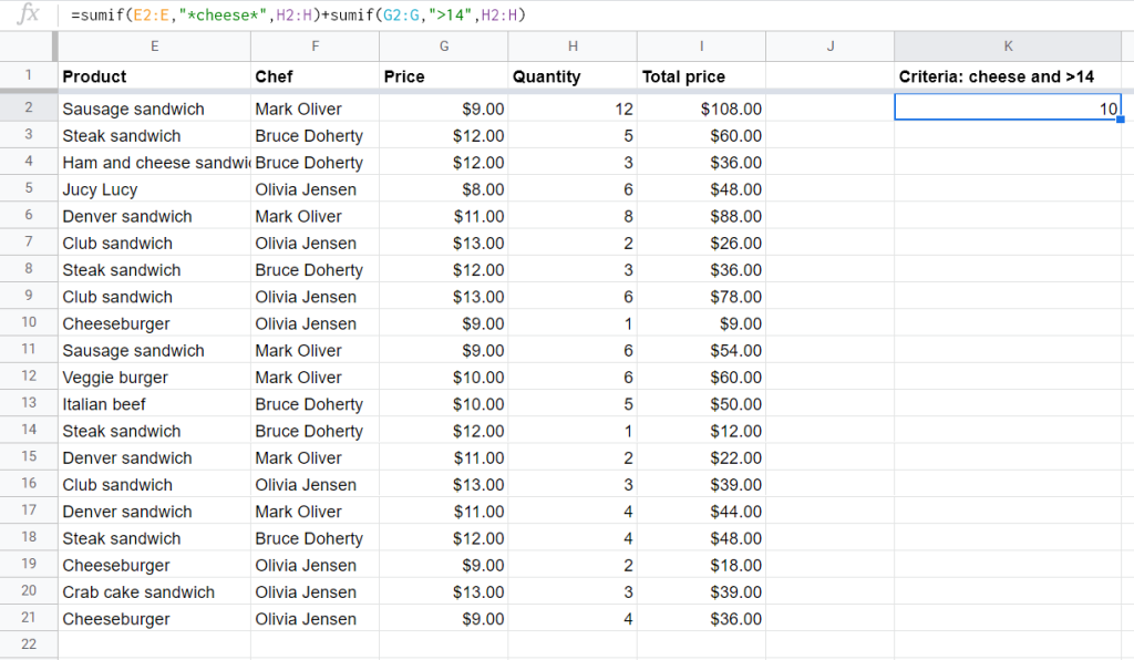
- Product name must contain “cheese“
- Product price must be greater than $14
As you can see, none of the products in our data set has the price greater than $14. So, the SUMIF formula returns the sum of values that match the first criterion only:
=sumif(E2:E,"*cheese*",H2:H)+sumif(G2:G,">14",H2:H)
SUMIF Google Sheets formula when any of multiple criteria is met
For multiple criteria within a single range, it’s not handy to use the approach above. So, you’d better use the following formula syntax:
=SUM(ARRAYFORMULA(SUMIF(criterion-range, {"criterion1", "criterion2", "criterion3"}, range-to-sum)))Note: The formula works for a single criterion-range only.
For example, we need to sum the values by one of the following product price criteria:
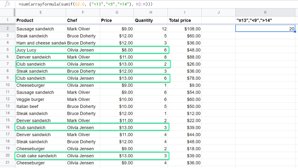
- Equal to $13
- Less than $9
- Greater than $14
Here we go:
=sum(arrayformula(sumif(G2:G, {"=13","<9",">14"}, H2:H)))
To wrap up: How to learn the sum without any formulas in Google Sheets
You’ve read the article till the end?! You’re a person of worth and deserve a tiny bonus. If you need to learn the total of specific cells right here, right now, you don’t need any formulas at all. Simply select the cells you want to sum and check out a new tab that appeared near the Explore button. Here is your total sum!
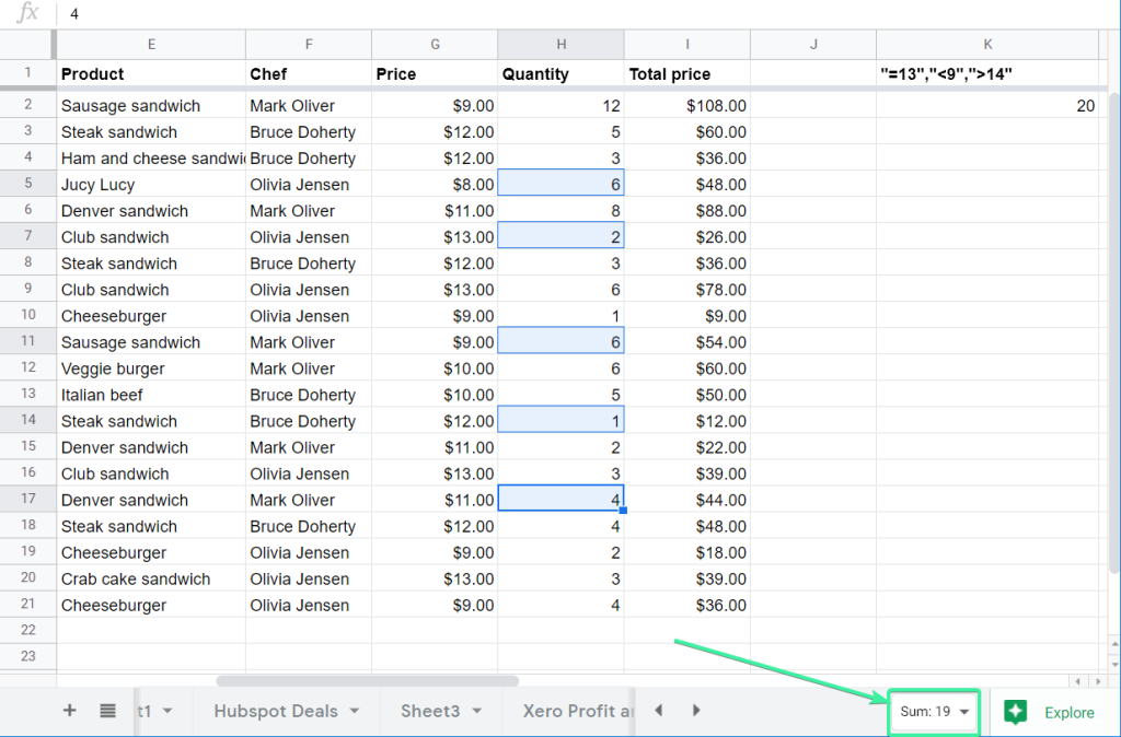
Quite handy, isn’t it? Good luck with your data!