Do you have a Google spreadsheet with structurally identical sheets and need to combine data from them? If so, there are versatile options to automate the flow and forget about manual work. Let’s explore several functions and a formula-free solution to merge sheets into one.
You can also check our video tutorial on the Coupler.io Academy YouTube channel.
Merge Google Sheets fast and without any formulas
To combine sheets automatically on schedule or just avoid formulas in Google Sheets to link to another sheet, use Coupler.io. It’s a reporting automation platform that allows you to import data between sheets in minutes. You can pull a data range from multiple sheets or merge them all together. Here’s how you can do this step by step:
- Get started by clicking Proceed in the interactive form below.
- Sign in to Coupler.io for free (no credit card required). Next, connect your Google account and select the necessary spreadsheet from your Google Drive and the sheets you’ll merge.
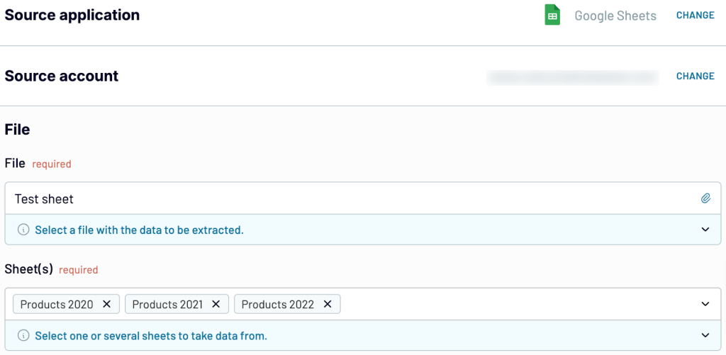
The order of the sheets specified doesn’t influence the order of the merged data. If you need to merge data in a specific order (for example, first Products 2020, then Products 2021, and Products 2022), make sure to arrange the sheets in your spreadsheet in this order.
- Once you’ve configured your source settings, move forward. Next, you can preview the data from the sheets to be merged and apply the necessary transformations, such as:
- Rename, rearrange, hide, or add columns.
- Apply filters and sort your data.
- Create new columns with custom formulas, etc.
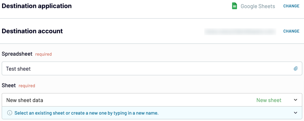
- When you’re ready with your data, proceed to connect your Google account, specify the spreadsheet, and select the sheet that will receive the combined sheets.
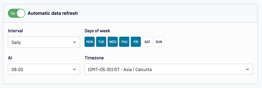
Then, you can automate reporting on schedule by turning on the Automatic data refresh. Specify an update interval from every month to daily and even every 15 minutes (that will make your report near real-time).
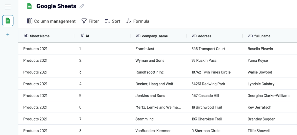
Finally, save and run the importer. Here’s what you’ll get:
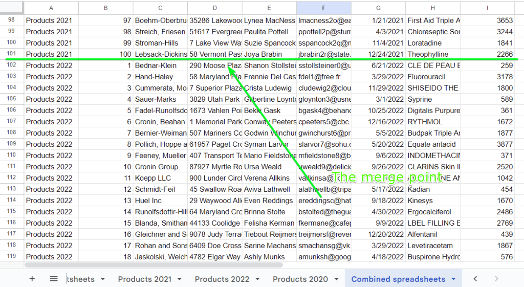
Coupler.io adds the Sheet Name column so you can easily navigate the merged Google Sheets.
Google Sheets to Google Sheets is not the only integration provided by Coupler.io. It also allows you to import data from CSV files, Excel files, and numerous apps.
Merge sheets with a patterned name
Imagine that you need to add more sheets in the future to merge data from and their names have the same pattern. Coupler.io enables you to use a pattern, regular expression, instead of manually selecting the sheet name from a list. This means new sheets matching your pattern will be imported automatically.
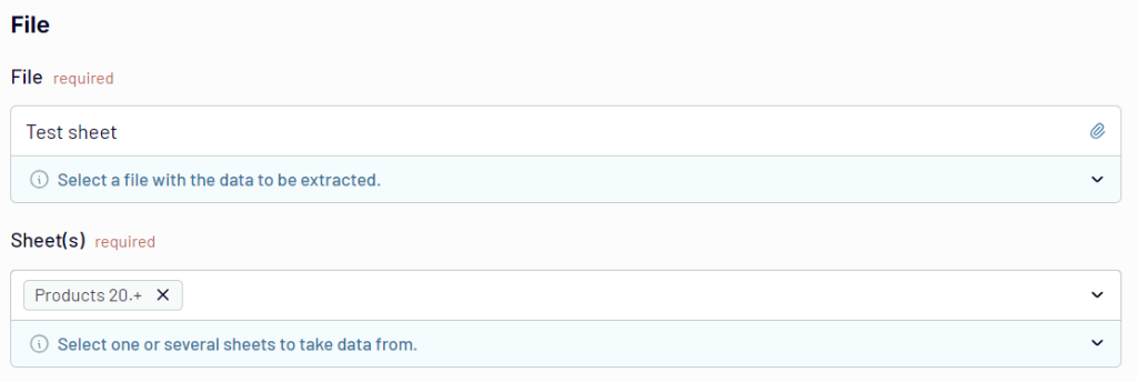
For example, your sheets with product items for the next 10 years are named as Products 2025, Products 2026, Products 2027, etc. Instead of typing in all of them one by one, use the {sheet-name}.+ pattern:
In our case, it will look as follows:Products 20.+
You can use the regular expressions for other cases. Here are the most common ones:
Match all sheets:
- Pattern:
.*
Match sheets by year:
2021.+matches: 2021-01, 2021-02, 2021-03, etc.202.+matches: 2020-12, 2021-01, 2021-02, 2022-03, etc..*202.matches: Dec 2020, Jan 2021, Feb 2021, All 2020, 12-2020, 01-2021
Match sheets by name prefix (starts with):
sales data.+matches all sheets with names that start with sales data
Match sheets by name content (contains):
.*sales data.*matches all sheets with names that contain sales data anywhere
Match sheets by name suffix (ends with):
.*sales datamatches all sheets with names that end with sales data
How to combine data from multiple sheets in Google Sheets with formulas
If you prefer the native options to combine sheets in Google Sheets, then let’s check them out below. Let’s begin with a simple task:
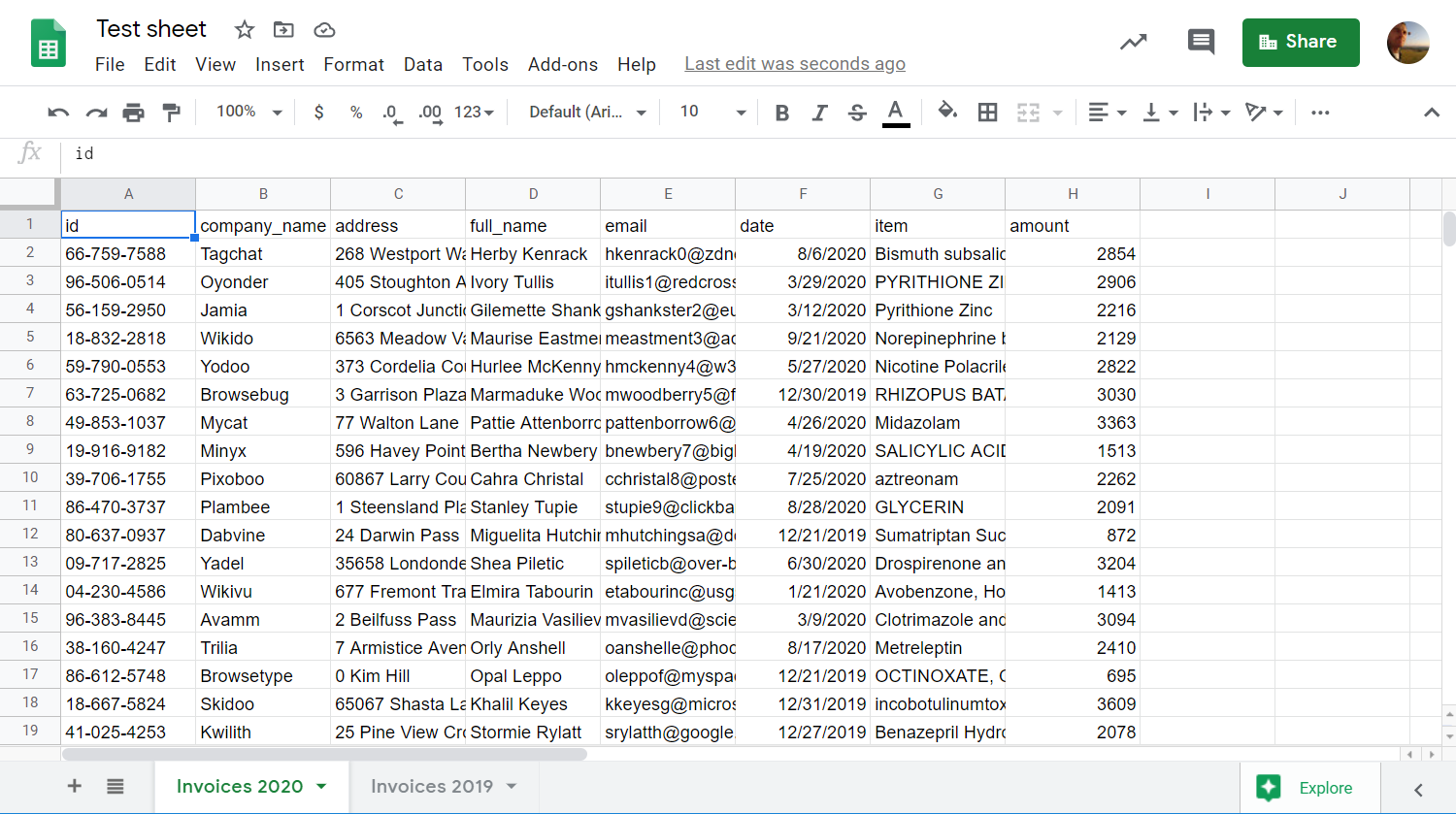
There is a Google Sheets doc with two sheets: Invoices 2019 and Invoices 2020. Each of these sheets has eight columns (A:H) of the same name. The first row contains the column titles. Our task is to merge data vertically from these sheets into one.
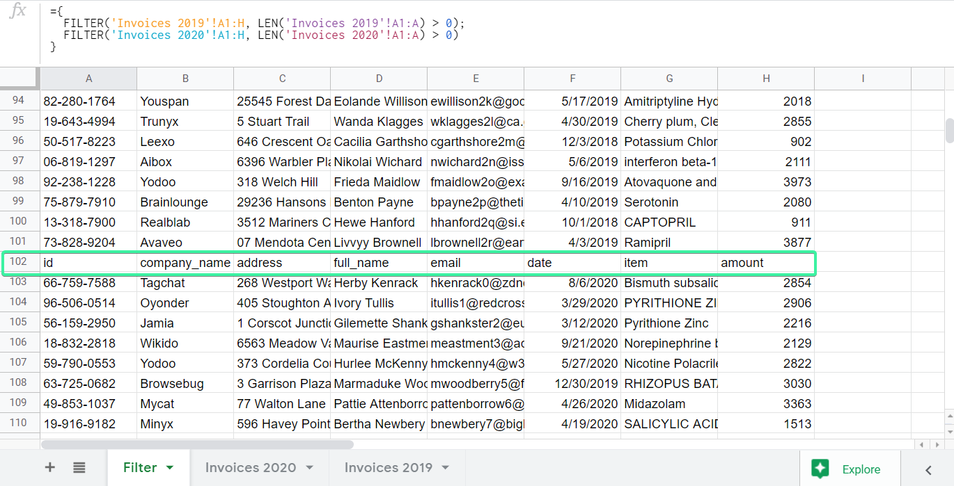
Use FILTER in Google Sheets
FILTER is a Google Sheets function that filters out subsets of data from a specified data range by a provided condition.
To combine sheets using FILTER, apply the following formula:
={FILTER({sheet#1-range},LEN({sheet#1-range-first-column})>0);
FILTER({sheet#2-range},LEN({sheet#2-range-first-column})>0);...}
{sheet#1-range}– the data range from the first sheet including the title row.{sheet#2-range}– the data range from the second sheet without the title row.{sheet#1-range-first-column}– the first column of the data range from the first sheet.{sheet#2-range-first-column}– the first column (without the title row) of the data range from the second sheet.
The LEN condition (LEN({sheet#1-range-first-column})>0) in the FILTER formula is required to skip empty rows in the range. Otherwise, the formula will also add empty rows when merging the rows with data.
In our case, the formula will look as follows:
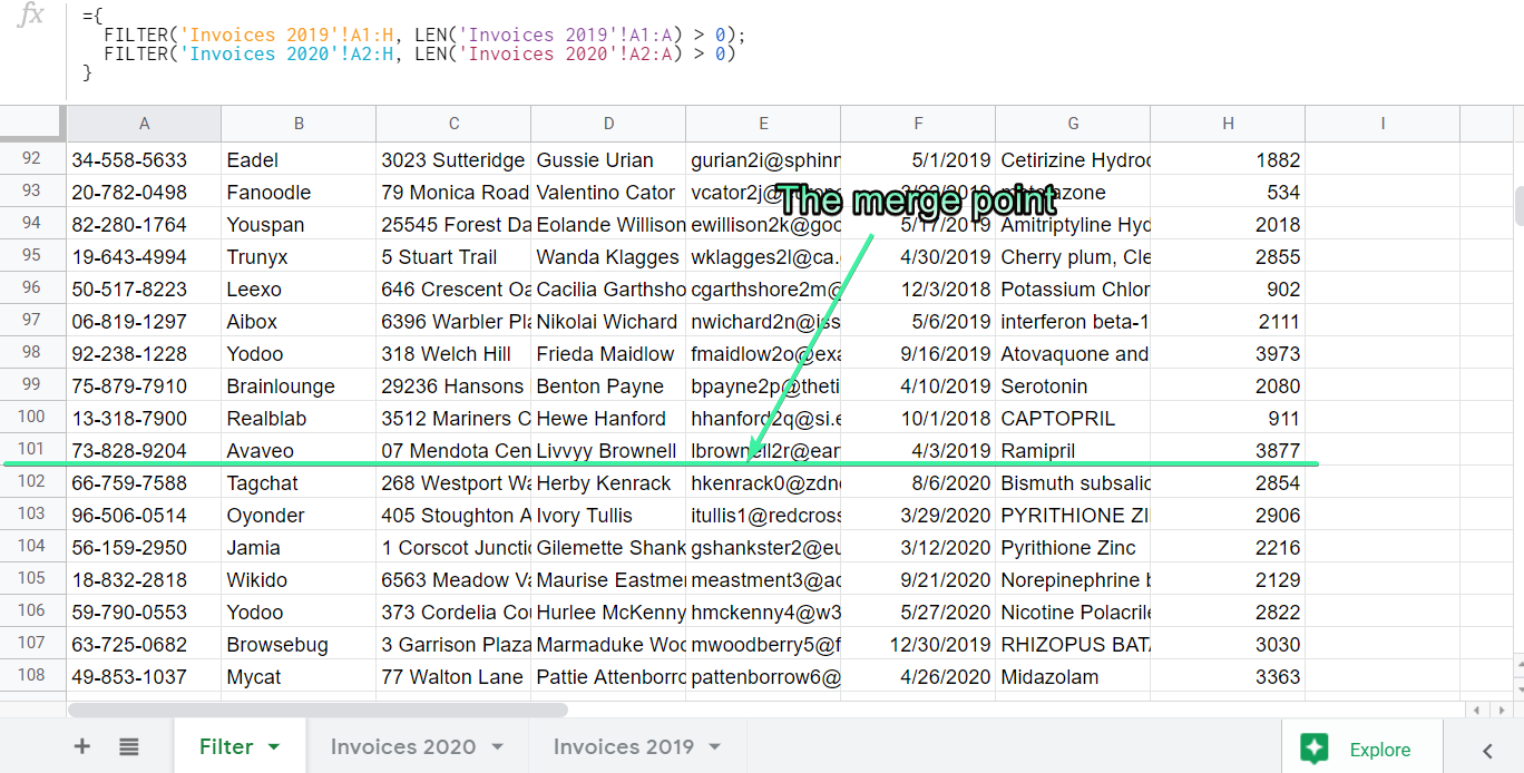
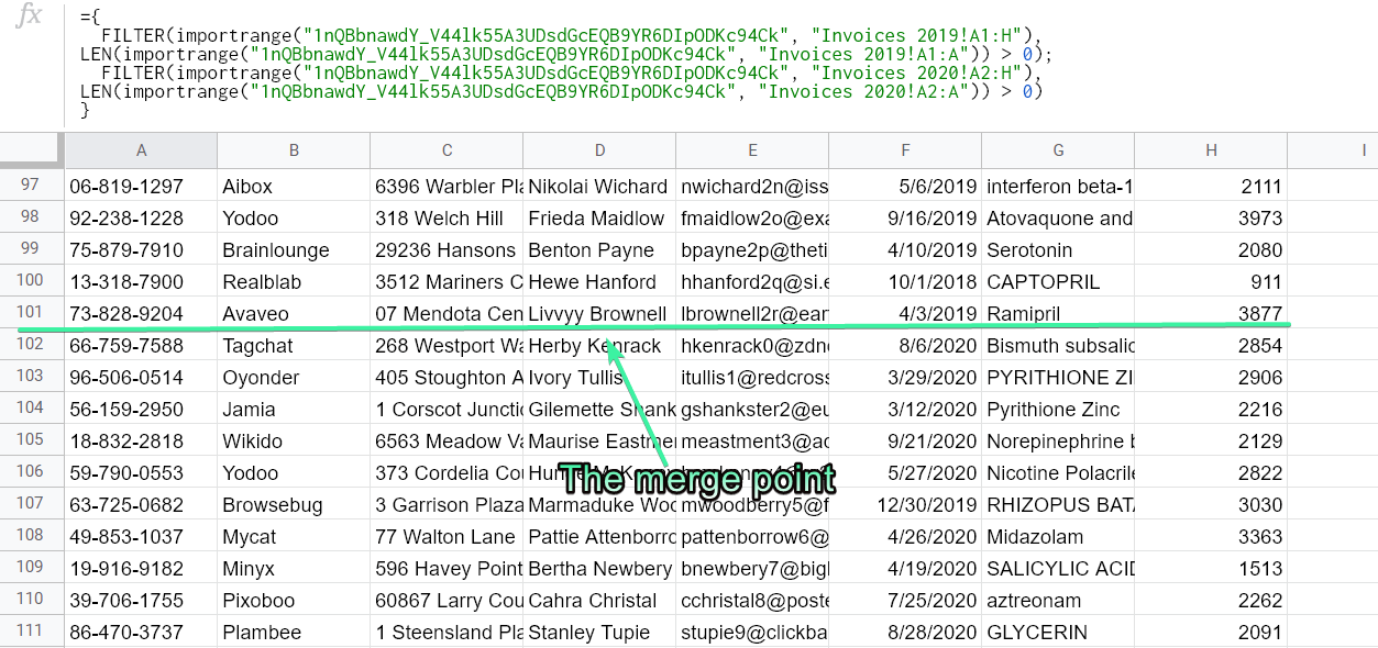
={
  FILTER('Invoices 2019'!A1:H, LEN('Invoices 2019'!A1:A) > 0);
  FILTER('Invoices 2020'!A2:H, LEN('Invoices 2020'!A2:A) > 0)
}
In this way, you can merge more than two sheets together. All you need to do is add relevant sheets and their ranges in the formula.
Note: Make sure to specify the data range from the second sheet (and subsequent ones) without the title row, such as A2:H instead of A1:H. Otherwise, the title row will also be imported. For example,
={
  FILTER('Invoices 2019'!A1:H, LEN('Invoices 2019'!A1:A) > 0);
  FILTER('Invoices 2020'!A1:H, LEN('Invoices 2020'!A1:A) > 0)
}
For more on how it works, read this FILTER Function How-to Guide.
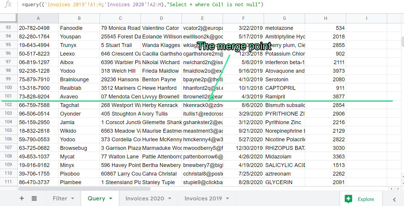
Use QUERY in Google Sheets
QUERY is a Google Sheets function to fetch the data based on specified criteria. Additionally, you can amend formatting, change the order of columns, and perform other manipulations with the imported data.
To combine sheets using QUERY, apply the following formula:
=QUERY({{sheet#1-range};{sheet#2-range};...,"Select * where Col1 is not null")
{sheet#1-range}– the data range from the first sheet including the title row.{sheet#2-range}– the data range from the second sheet without the title row.
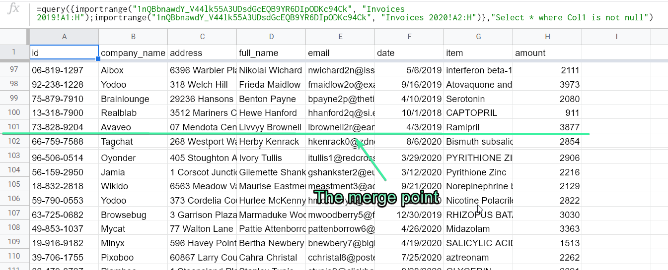
In our case, the formula will look as follows:
=query({'Invoices 2019'!A1:H;'Invoices 2020'!A2:H},"Select * where Col1 is not null")
You can merge more than two sheets together with QUERY if you add relevant sheets and their ranges in the formula. Don’t forget that the ranges from the second and subsequent sheets should be specified without the title row, just like with the FILTER function above.
Mind that the mentioned QUERY and FILTER formulas merge sheets with the same number of columns only. For other cases, read our guide on How To Combine Sheets With a Different Number of Columns Into One.
Here is the list of most common cases:
Match all sheets:
- Pattern:
.*
Match sheets by year:
2021.+matches: 2021-01, 2021-02, 2021-03, etc.202.+matches: 2020-12, 2021-01, 2021-02, 2022-03, etc.- `.*202. matches: Dec 2020, Jan 2021, Feb 2021, All 2020, 12-2020, 01-2021
Match sheets by name prefix (starts with):
sales data.+matches all sheets with names that start with “sales data”
Match sheets by name content (contains):
.*sales data.*matches all sheets with names that contain “sales data” anywhere
Match sheets by name suffix (ends with):
.*sales datamatches all sheets with names that end with “sales data”
Combine sheets into one and consolidate data using QUERY
We’ve successfully combined sheets with invoice data. However, it would be great if we could not only merge but also consolidate data in Google Sheets. For example, the invoice amount of the Abatz company in 2020 was $1778, and it was $2864 in 2019. The Abatz’s total invoice amount is $4642.
Our goal is to consolidate the invoice amount for all companies that have records on both sheets. For this, we’ve modified the QUERY formula above to get the following:
=query({'Invoices 2019'!A1:H;'Invoices 2020'!A2:H},"Select Col2,sum(Col8) where Col1 is not null group by Col2")
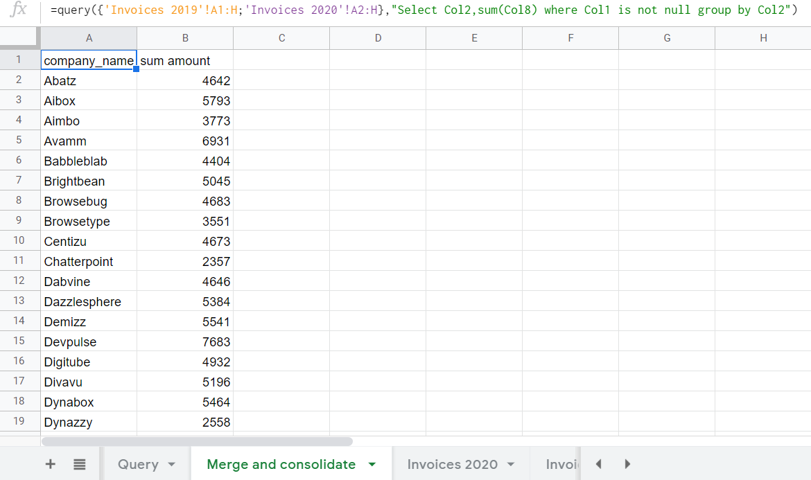
Since company_name is the only iterative parameter for which we are consolidating data, we do not need to query other columns from the sheets. Read the QUERY How-To Guide to learn more.
How to merge sheets from another Google Sheets spreadsheet/workbook without formulas
We already know how to combine sheets within a Google Sheets workbook. Now let’s explore how you can import two or more sheets from another spreadsheet and merge them into one.
I have a spreadsheet on my personal Google account – let’s name it External spreadsheet. I need to import and merge two sheets (Invoices 2019 and Invoices 2020) from the spreadsheet that has been featured in the examples above. This spreadsheet is on my working Google account. We’ll check out all possible options, and the no-formula one will be first.
Coupler.io and its Google Sheets integration is the most actionable way to import and merge data from a Google Sheets workbook. We’ve described the setup flow above. In brief, it looks as follows:
- Click Proceed in the form below:
- Connect your Google account, then select a file on your Google Drive and sheets that you want to merge.
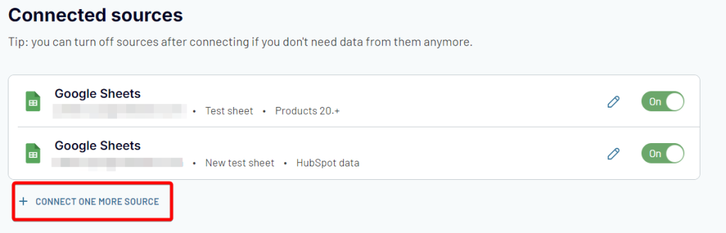
- Then click Connect one more source, select Google Sheets, and specify another workbook and the sheet(s) you want to combine. This way, you can add multiple Google Sheets documents you want to combine.
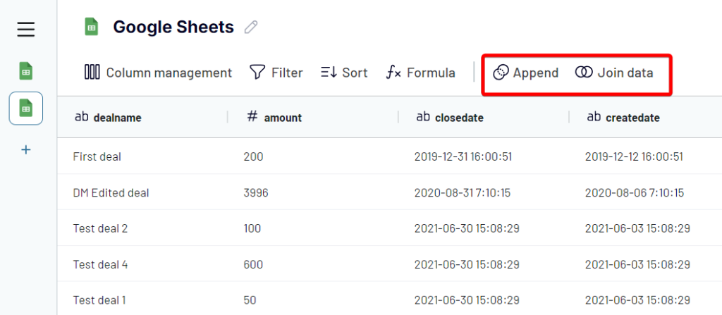
- After setting up your source, proceed to the next step preview the data and choose how you want to merge your data and make transformations if needed. Coupler.io lets’ you append or join data:
- Append data if you need to combine sheets with identical structures.
- Join data if you need to merge sheets with different structures.
- Next, connect your Google account, then select the destination spreadsheet and a sheet to transfer the merged data.
- Lastly, configure your data refresh schedule and run the importer.
Use formulas to merge sheets from different Google Sheets docs
You can do the same using QUERY or FILTER formulas nested with IMPORTRANGE. It is a function that allows you to import a data range from one Google Sheets document to another. Read the IMPORTRANGE tutorial to learn more about it.
Another use case is when you need to merge a sheet from one Google Sheets doc and a sheet from another Google Sheets doc. You can easily handle this using either FILTER+IMPORTRANGE or QUERY+IMPORTRANGE. The difference is that you’ll have to specify different spreadsheet IDs in the respective parameters of the IMPORTRANGE formula.
Use FILTER + IMPORTRANGE
The FILTER+IMPORTRANGE formula syntax to combine two or more sheets from another spreadsheet is the following:
={FILTER(IMPORTRANGE("{spreadsheet-ID}", "{sheet#1-name}!{sheet#1-range}"),LEN(IMPORTRANGE("{spreadsheet-ID}", "{sheet#1-name}!{sheet#1-first-column})>0);
FILTER(IMPORTRANGE("{spreadsheet-ID}", "{sheet#2-name}!{sheet#2-range}"),LEN(IMPORTRANGE("{spreadsheet-ID}", "{sheet#2-name}!{sheet#2-first-column})>0);...}
{spreadsheet-ID}– the ID or URL of the Google Sheets document you’re importing data from{sheet#-name}– the name of the sheet{sheet#-range}– the data range from the sheet including the title row.{sheet#-first-column}– the first column of the data range from the sheet.
This is how the formula looks for our use case:
={
  FILTER(importrange("1nQBbnawdY_V44lk55A3UDsdGcEQB9YR6DIpODKc94Ck", "Invoices 2019!A1:H"), LEN(importrange("1nQBbnawdY_V44lk55A3UDsdGcEQB9YR6DIpODKc94Ck", "Invoices 2019!A1:A")) > 0);
  FILTER(importrange("1nQBbnawdY_V44lk55A3UDsdGcEQB9YR6DIpODKc94Ck", "Invoices 2020!A2:H"), LEN(importrange("1nQBbnawdY_V44lk55A3UDsdGcEQB9YR6DIpODKc94Ck", "Invoices 2020!A2:A")) > 0)
}
Merge cells in Google Sheets with QUERY + IMPORTRANGE
The QUERY+IMPORTRANGE formula syntax to combine two or more sheets from another spreadsheet is shorter:
=QUERY({IMPORTRANGE("{spreadsheet-ID}", "{sheet#1-name}!{sheet#1-range}");IMPORTRANGE("{spreadsheet-ID}", "{sheet#2-name}!{sheet#2-range}");...,"Select * where Col1 is not null")
{spreadsheet-ID}– the ID or URL of the Google Sheets document you’re importing data from{sheet#-name}– the name of the sheet{sheet#-range}– the data range from the sheet including the title row.
In our case, the formula will look as follows:
=query({importrange("1nQBbnawdY_V44lk55A3UDsdGcEQB9YR6DIpODKc94Ck", "Invoices 2019!A1:H");importrange("1nQBbnawdY_V44lk55A3UDsdGcEQB9YR6DIpODKc94Ck", "Invoices 2020!A2:H")},"Select * where Col1 is not null")
IMPORTRANGE #REF! You need to connect these sheets
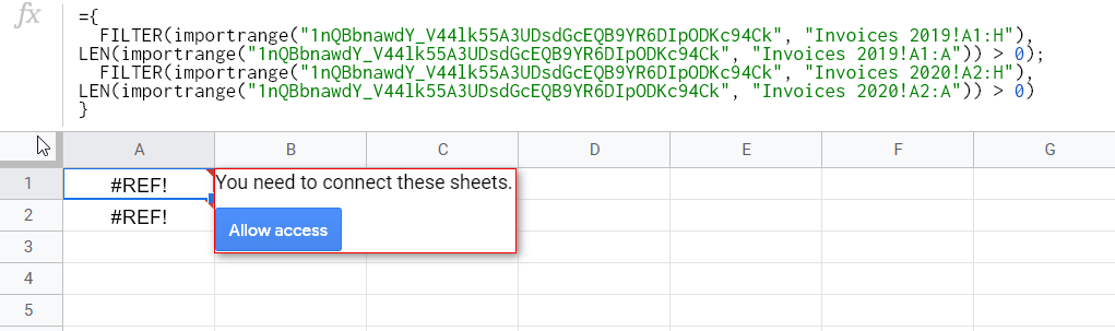
It’s OK if you’ve got this warning during the initial run of either FILTER+IMPORTRANGE or QUERY+IMPORTRANGE formula. Click Allow access to connect the source and target spreadsheets. After that, the formula will import and merge Google Sheets. If you’ve got another error, check out our blog post Why IMPORTRANGE Is Not Working: Errors and Fixes.
Which option is best to combine Google Sheets?
FILTER
The FILTER function is good when you need to merge sheets within a single spreadsheet. It’s simple and doesn’t require any advanced knowledge. At the same time, the syntax of FILTER nested with IMPORTRANGE is quite voluminous, so you’d better avoid using FILTER for merging sheets from external spreadsheets.
QUERY+IMPORTRANGE
The combination of QUERY and IMPORTRANGE is the best choice to consolidate data in Google Sheets. Its syntax is easy to comprehend and is not as bulky as with FILTER.
Google Sheets integration by Coupler.io
If you don’t want to waste time writing formulas and checking their syntax, go with the Google Sheets integration by Coupler.io. It’s easy to use and allows you to schedule data import & merge. The integration is especially functional if you need to combine multiple sheets from other Google Sheets spreadsheets. In this case, it’s an advanced alternative to the IMPORTRANGE function.
Besides, with Coupler.io, you can import data from 70+ cloud apps into a single spreadsheet for further processing. For example, here is how you can apply it to merge Excel sheets.

Import and combine data in Google Sheets with Coupler.io
Get started for free